Conditional Formatting Highlighting Random Cells

[LL19911695]

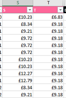
I am trying to set up some simple conditional formatting in Excel; I want cells in column S to turn red where S is less than T. (See below.)

Below is a screenshot of the formula I am using:

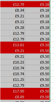
However, using this formula, Excel appears to be highlighting random cells:

FYI - column S is actually a formula (=N20/52.14/P20) and column T is a VLOOKUP, however

[#2]

@LL19911695 

=$S$2:$T$1048576

Apply the conditional format to the above range and it will work.

Currently your rule for conditional formatting starts in row 2 and the format is applied from row 1 (=$S:$T) and therefore the format is applied 1 row above.