Conditional Formatting Help!!!

[jringerwalshgroupcom]

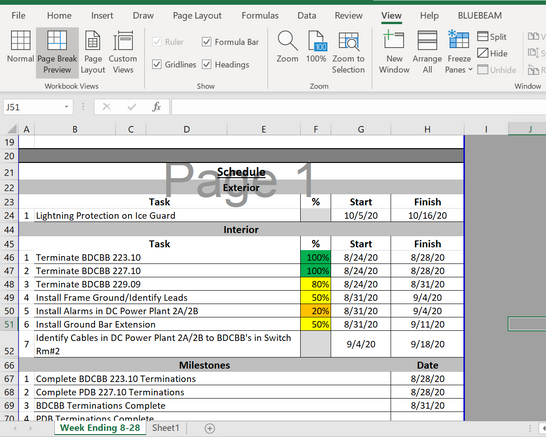
How do I get rows 46-52 to have the same rules as column F? I want the rows to be highlighted the same color as column F. Any help would be greatly appreciated.  

   

[#2]

@jringerwalshgroupcom 

Select the range in rows 46 to 52 that you want to format (or the entire rows if you wish).

I will assume that the active cell in the selection is in row 46.

On the Home tab of the ribbon, select Conditional Formatting > New Rule...

Select 'Use a formula to determine which cells to format'.

Enter the formula =$F46>0%

Click Format...

Activate the Fill tab.

Select orange.

Click OK, then click OK again.

Repeat the above steps, but with =$F46>20% and yellow.

Repeat them again but with =$F46>80% and green.

If necessary, change the thresholds (you didn't tell us what your conditional formatting rules are).