Conditional Formatting help!

[yejinshim]

Hello community,

I'm trying to figure out how to utilize the conditional formatting feature for my sheet.

This is what a part of my data looks like:

I want the "Average" columns to highlight in a red box if the values are less than 3.5 (for example). As you can see, the "Average" columns can be found in columns M, N, and O and I only want to highlight the values of "Average" in columns M, N, and O, and nothing else.

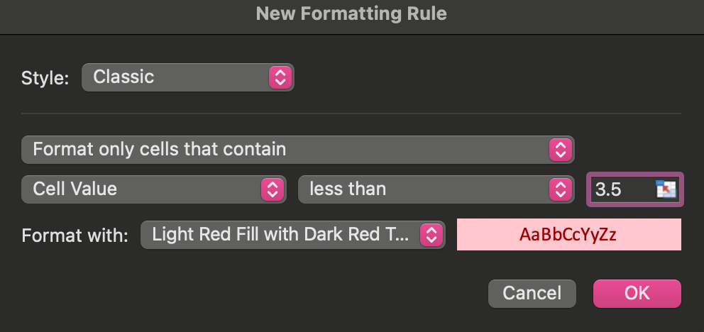
But when I try selecting all columns M, N, and O and apply conditional formatting "Highlight Cells Rules" > "Less Than" and select below:

Then, this is what happens:

- What do I need to do if I don't want to highlight the boxes with no value (empty boxes)?
- What do I need to do if I don't want it to highlight the "Percent" values? I want "Average" only.

If you know how to work with this feature, please guide me on the path! Thank you so much in advance!

[#2]

@yejinshim 

Select only M8:M11, N17:N26 and O32:O33 when you create the rule.

[#3]

Hi Hans,

Thank you. That's a good way when you work with small data (manually selecting each section). However, I'm here dealing with hundreds of data like this and the screenshot I posted is just a part of it and it's impossible for me to go down the data and manually select like this. I was hoping to see if there's a way to do this in an easier way when dealing with huge chunks of data.

Thank you!

[#4]

@yejinshim 

I'm afraid you'll have to do that...