- Home
- Microsoft 365
- Excel
- Re: Conditional Formatting Formula for Dates
Conditional Formatting Formula for Dates
- Subscribe to RSS Feed
- Mark Discussion as New
- Mark Discussion as Read
- Pin this Discussion for Current User
- Bookmark
- Subscribe
- Printer Friendly Page
- Mark as New
- Bookmark
- Subscribe
- Mute
- Subscribe to RSS Feed
- Permalink
- Report Inappropriate Content
Apr 26 2021 01:58 PM
Hello!
I am trying to write a formula for conditional formatting to be applied to two columns with dates. Column B is the Next Shipment Date, and Column C is the Due Date of the order. I have other conditional formatting to highlight in both columns if the date has passed.
Now, I'm trying to use conditional formatting to highlight cells in Column B if the following criteria are met:
1. If the Next Shipment Date is AFTER the Due Date
AND 2. If the Due Date is NOT blank
3. If the Next Shipment Date IS blank
Item 3 may need to split into its own conditional formatting rule, which is fine. However, I think items 1 & 2 need to be combined into one formula to identify the proper fields.
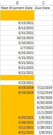
The screen shot below is from my data showing that there are rows in which the Next Shipment Date or Due Date (or both) are blank. I removed other conditional formatting from this sample.

The screen shot below shows what I would like to highlight based on the criteria detailed above.
I have scoured Excel forums looking for a solution and haven't been able to come up with anything that works the way I need it to. I'm not new to Excel, but I don't have much experience (yet) with writing formulas with multiple conditions/criteria. It's also possible I'm just overthinking this. Any help is much appreciated!! Thanks in advance!
- Labels:
-
Excel
-
Formulas and Functions
- Mark as New
- Bookmark
- Subscribe
- Mute
- Subscribe to RSS Feed
- Permalink
- Report Inappropriate Content
Apr 26 2021 02:17 PM
Select B2:B200 (or however far down the data go).
B2 should be the active cell in the selection.
On the Home tab of the ribbon, select Condtional Formatting > New Rule...
Select 'Use a formula to determine which cells to format'.
Enter the formula
=OR(AND(C2<>"",B2>C2),B2="")
Click Format...
Activate the Fill tab.
Select a color.
Click OK, then click OK again.
- Mark as New
- Bookmark
- Subscribe
- Mute
- Subscribe to RSS Feed
- Permalink
- Report Inappropriate Content
Apr 26 2021 02:54 PM
Thank you for your response! This works in my sample data sheet, but does not work in my regular data sheet.
Below is the current conditional formatting rules for the worksheet. I think something is interfering. I also included a screenshot of the subject cells with current conditional formatting rules. Not sure where to go from here.
I am trying to do the following:
- Block empty cells and text cells from any conditional formatting
- Highlight in red cells that are "late" / equal to or past today's date
- Highlight in yellow cells that are "upcoming" / equal to or within next 14 days
- And from my original post, highlight in orange cells with next shipment date that is after the due date
AC is Next Shipment Date
In the screenshot below, it looks like the orange formatting is overruling the "late" and "upcoming" formats.
- Mark as New
- Bookmark
- Subscribe
- Mute
- Subscribe to RSS Feed
- Permalink
- Report Inappropriate Content
Apr 26 2021 03:19 PM
@VICTORIAR94 Try moving the rule for orange down to below the rules for red and yellow.
- Mark as New
- Bookmark
- Subscribe
- Mute
- Subscribe to RSS Feed
- Permalink
- Report Inappropriate Content
Apr 27 2021 05:53 AM
Orange rule is now at the bottom but the highlighted cells did not change.
- Mark as New
- Bookmark
- Subscribe
- Mute
- Subscribe to RSS Feed
- Permalink
- Report Inappropriate Content
Apr 27 2021 05:57 AM
Could you attach a small sample workbook without sensitive data that demonstrates the problem?
- Mark as New
- Bookmark
- Subscribe
- Mute
- Subscribe to RSS Feed
- Permalink
- Report Inappropriate Content
Apr 27 2021 06:06 AM
Sample attached below. Thank you again for your help!!


