Conditional formatting for x number of days before

[Rick151]

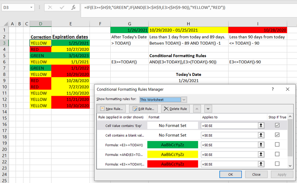
I am trying to set a conditional formatting for an expiration date field. The idea is to show via color coding (green, yellow, and red) when the expiration date is approaching according to the cell (In the E column) and today's date.

It should fill green when the date in the field is equal or after today

=E3>TODAY()

 

It should fill yellow when the date in the field is less than today and less than 3 months (90 days) (between 89 days and yesterday)

=AND(E3<TODAY(),E3>(TODAY()-90))

 

It should fill red when the date in the field is less than 3 months (90 days)

=E3<=TODAY()-90

I have included the dates (including "today's date") as reference. 

I added the Conditional Formatting Rules formula in the cells. 

I also included the Correction column to show what the correct color should be.

The colors do not match my date ranges.

[#2]

@Rick151 

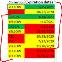
When you enter the conditional format formulas, remember that the cell addresses of the conditional format formula are relative to the active cell. Is it possible you had cell E1 as the active cell when you entered the conditional formats? Notice how your formats are off by 2 rows (move your correct column up two cells and they match)?

[#3]

@JMB17

I had tried deleting the top rows still the same. I uploaded my file.

[#4 · Accepted solution]

@Rick151 so as @JMB17 indicated your reference is wrong.  Your 'Applies to' field is $E:$E which means your top left most cell is E1 but your formulas all use E3 which is why everything is off by 2 rows.  You can change the formulas to use E1 and it will work.

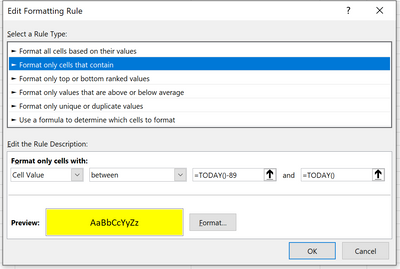
That said, you could also just use the built in conditional formatting:

and then you don't need any cell references.

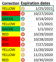
And alternative solution instead of having 3 conditional formatting rules you can use ICON sets instead:

  

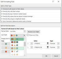
a different look which may or may not be good for what you want.

[#5]

@Rick151 

No, deleting the top rows won't fix it. You have to edit the formulas.

The formulas apply to the range E:E and the cell references of your formulas are relative to the top left cell of the 'applies to' range (so cell E1 in this case). Your formulas reference cell E3, which is 2 rows down from cell E1. So, the formula will be looking at the value of E5 when it's evaluating the conditional format of cell E3 (and so on).

Try changing the formulas to:

Green: =E1>=TODAY()

Yellow: =AND(E1<TODAY(),E1>(TODAY()-90))

Red: =E1<=TODAY()-90

[#6]

@mtarler 

It all came down to that I was selecting the wrong rule type.

I changed the rule type from Use a formula to determine which cells to format to Format Cells that contain and it worked perfectly.

Thanks!