Conditional Formatting - Consider Only Value as Lowest Value

[Ben Smith]

When "Formatting Cells Based on Value" if there is only one cell with data out of a set of otherwise blank cells, the rule considers the existent data as highest value. This makes sense logically, but I want the lowest value, even if it is the only value, to display as such. I can't figure out how to use another rule to eliminate the blank cells from the value-based rule. Thanks in advance!

[#2 · Accepted solution]

Hi Ben,

More exactly blank cells are ignored in any case. If you have only one value it is simultaneously min and max value in the range, Excel goes from min to max and shows you that one number as the biggest one.

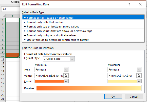
If you'd like to show it as the lowest you shall reverse "the axis" and if that is the only number add to it something compare reversed minimum, like this

where formula for minimum is

=MAX($A$1:$A$10)+(COUNTA($A$1:$A$10)=1)

and for maximum

=MIN($A$1:$A$10)

If you have more than one number colour grade will be correct (min is darker for our scale)

and attached

[#3]

I'll be honest, I don't understand how the above works, mostly due to the (COUNTA(x,y,z)=1) output being either TRUE or FALSE - I'm not sure how that affects the minimum formula. I also don't know how calling out the largest number in MIN and the smallest in MAX isn't reversing the color gradient (without my reversing the colors).

That said, it works beautifully. Thank you!