Conditional Formatting between certain dates

[NConde]

I have a date collumn and a number that was completed on that date. 

I want a forumla that will alert me if i try and put the same number on another row WITHIN 6 months of that first date.

Example: 

January 4th - 4201 

February 10th - 4201

I want it to highlight that because its WITHIN 6 months of each other.

Column information.

Date Column is C

Number Columns are F - O

[#2]

@NConde 

Assuming that your data begin on row 1:

Select F2:Kn where n is the last used row.

F2 should be the active cell within the selection.

Create a conditional formatting rule of the formula type with the following formula:

=SUMPRODUCT(($F$1:$K1=F2)*($C$1:$C1>=EDATE($C2,-6)))

[#3]

@Hans Vogelaar That didnt work, They didnt highlight if they were within 6 months. 

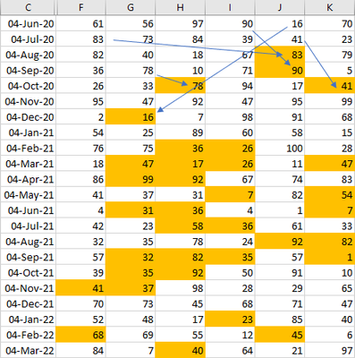
[#4 · Accepted solution]

@NConde 

This is what I get. I drew lines for the first occurrences.

Perhaps I misinterpreted your question. If so, please explain in more detail what you want.

 

[#5]

The formula is on my spreadsheet in 3 different sections, its working perfectly for 2 of the 3 locations, The 3rd location on the tracker the formula is almost upside down, Instead of highlighting the 2nd date being within 6 months, its highlighting the first date.

[#6]

@NConde 

Are the dates sorted differently in the 3rd section?

[#7]

Nope exactly the same, infact it uses the same date column as the other ones

First section
=SUMPRODUCT(($F$9:$O9=F10)*($C$9:$C9>=EDATE($C10,-5)))
Second section
=SUMPRODUCT(($Q$9:$V9=Q10)*($C$9:$C9>=EDATE($C10,-5)))
third section - section thats not working properly
=SUMPRODUCT(($X$9:$AA9=X10)*($C$9:$C9>=EDATE($C10,-5)))

[#8]

@NConde 

Could you attach a small sample workbook that demonstrates the problem, but without sensitive data?

[#9]

@Hans Vogelaar 

Here is a sample. I appreciate your assistance

[#10]

@NConde 

Thanks!

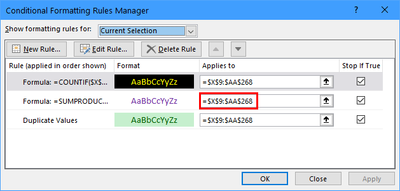
The difference is the range you've applied the rule to.

As for the columns to the left, the middle rule should start in row 10, i.e. it should apply to $X$10:$AA$268. Unfortunately, when you edit the Applies to box, the formula will change, so you'll have to make sure that it is

=SUMPRODUCT(($X$9:$AA9=X10)*($C$9:$C9>=EDATE($C10,-5)))

after the edit.

See the attached version.

[#11]

Thank you! this is now working! I appreciate all of your assistance!