conditional formatting based on cells with a formula

[A_Smit85]

For a project I need to use colours based on if something needs further steps yes or no (JA/NEE).

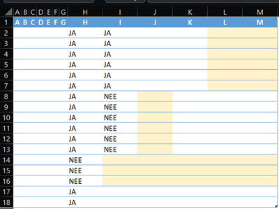
In the first picture you see the format I'd like to achieve. 

When Column H shows JA (yes), then column I till M should stay blank

When column H shows NEE (no), then column I till M should be filled

When Column H shows JA, and Column I shows JA, column L and M should be filled

When Column H shows JA, and Column I shows NEE, column J should be filled

However because a lot of formatting is based on column H, which shows a formula (see picture 2), I have some trouble.

In picture 3 you see the list of current rules in the table, this list goes on and on and on. Is it necessary for each cell to create a new rule?

If someone can point me in the right direction, I would be very grateful. The complete file is more than 1000 rows, and has more columns, but for readability I’ve selected but a few lines.

Thanks! 

[#2]

@A_Smit85 

IMHO some information is missing to make sure When column H shows NEE (no), then column I till M should be filled does what you expect => I assumed column I would equal to "" for that rule

[#3]

the examples I've attached to my request have been done by manually filling the cells, to show the example I was trying to reach. I'd like to change that to conditional formatting, so I don't have to do it manually for all rows.