Conditional Formatting based on a range of values

[Ahmed_Ezzedin]

Hi everyone,

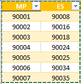
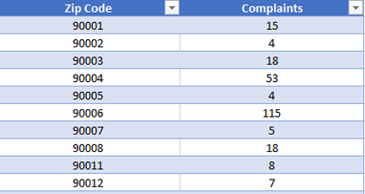
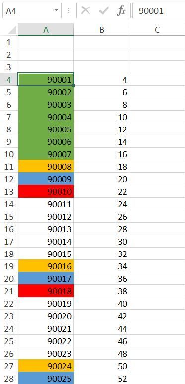
I'm trying to highlight rows in a table based on values of cells in another table in another worksheet (sheet1). Both tables contain zip codes, however, the table in sheet1 divides the zip codes by office. I want to highlight zip codes of each office with a different color. this the table I want to apply the conditional formatting to, values starts in A4 and B4

 This the table in Sheet1 where zip codes are divided by office. Data starts in A2, B2, C2, and D2 Thanks in advance for all you comments and assistance.

[#2]

@Ahmed_Ezzedin 

Is this what you are looking for?

[#3]

Yes, I'm pretty sure that the way you did it could be changed to highlight the whole row. Can please share with me how to apply it to my tables. :)

[#4]

@Ahmed_Ezzedin 

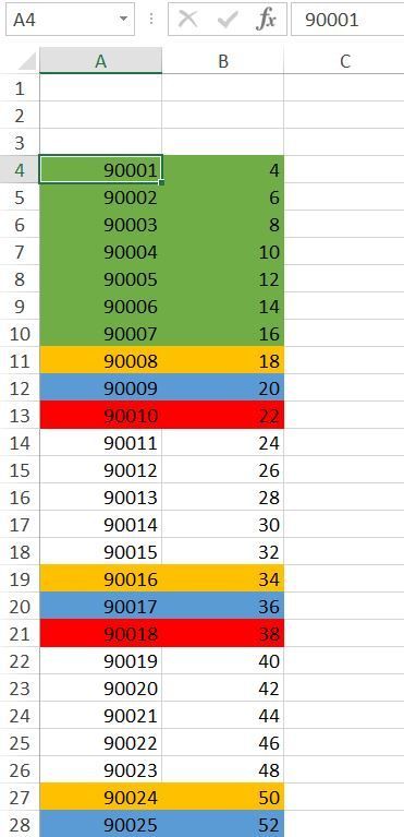
I changed the rule for conditional formatting from

=MATCH(A4,sheet2!$A$2:$A$8,0)

to

=MATCH($A4,sheet2!$A$2:$A$8,0)

The "applies to" range is =$A$4:$B$35

If you want to highlight e.g. columns A to H then change the "applies to" range to

=$A$4:$H$35

[#5]

THANK YOU VERY MUCH! It worked. Can you please explain the "0" in the match formula, so that I can use it in the future. <3

[#6]

@Ahmed_Ezzedin 

You are welcome. Glad my suggestion is helpful.

"0" is one of the match_types of the match function. You can read about it's behaviour here:

MATCH function (microsoft.com)