Conditional formatting based on a field below

[Wojciech_Plonka]

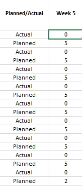
Hi, I have the following table:

Each actual value is relating to the "Planned" value below. I would like each "Actual" value to have a red colour if the planned value is 0 or green if the number is equal to the "Planned" value below. Each field can have a different planned value, so I need a smart formula.

Are they any ways to do it? Thank you

[#2]

@Wojciech_Plonka 

I tried to replicate what you ask for. Something like that?

[#3]

@Wojciech_Plonka 

Absolutely there are ways to do it.

If I were you, however, I'd put the cells side-by-side if you can. Makes it easier, and probably would make more sense design wise.

Anyway, here's an example. I used a random number generator just to put it through its paces. To get a whole new set of numbers, just activate the F9 key. With a mac that's done by holding the Fn key and pressing the key along the top row with F9 appearing on it.

[#4]

@Wojciech_Plonka 

Hi

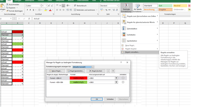
I think this might be what you want? This uses conditional formatting and might help you?

BTW - is there any reason why you have to layout with actual above planned? If you have actual next to planned (as shown on the right hand side) that it is easier to understand and the formatting also is simpler.

hope this helps.

Peter

[#5]

You and I think alike. I made the same recommendation: change to side-by-side!

[#6]

Well, the trick is - there will be thousands of rows like this, so setting this up manually would be a hell, also, changing format is impossible unfortunately


@PhilipTx @mathetes @peteryac60 

[#7]

@Wojciech_Plonka 

Yes, my solution would probably only work in a limited environment and was a basic attempt to understand your issue. If you apply the rule itself to the first rows you just got just replicate the format.  I can then only recommend to try a solution with visual basics. I used that in certain applications.   

Example for visual basics: 

Sub Kontrollkästchen61_Klicken()
If ActiveSheet.Shapes("Kontrollkästchen 61").OLEFormat.Object.value = 1 Then

Range("M67").Interior.ColorIndex = 6

Else
Range("M67").Interior.ColorIndex = xlNone

End If
ganzeZeile
End Sub
Sub Kontrollkästchen62_Klicken()
If ActiveSheet.Shapes("Kontrollkästchen 62").OLEFormat.Object.value = 1 Then

Range("N67").Interior.ColorIndex = 6

Else
Range("N67").Interior.ColorIndex = xlNone

End If
ganzeZeile
End Sub
Sub Kontrollkästchen63_Klicken()
If ActiveSheet.Shapes("Kontrollkästchen 63").OLEFormat.Object.value = 1 Then

Range("O67").Interior.ColorIndex = 6

Else
Range("O67").Interior.ColorIndex = xlNone

End If
ganzeZeile
End Sub
Sub ganzeZeile()

If ActiveSheet.Shapes("Kontrollkästchen 61").OLEFormat.Object.value = 1 And ActiveSheet.Shapes("Kontrollkästchen 62").OLEFormat.Object.value = 1 And ActiveSheet.Shapes("Kontrollkästchen 63").OLEFormat.Object.value = 1 Then

Range("A66:L68").Interior.ColorIndex = 6

Else

Range("A66:L68").Interior.ColorIndex = xlNone

End If
End Sub

There are likely more elegant or sophisticated approaches for this, but that would be a way to adress your issue. In future Excel will open up even further.