Conditional formatting based off two variables - SOLVED

[SamMitchell515]

Hi! My first time posting :)

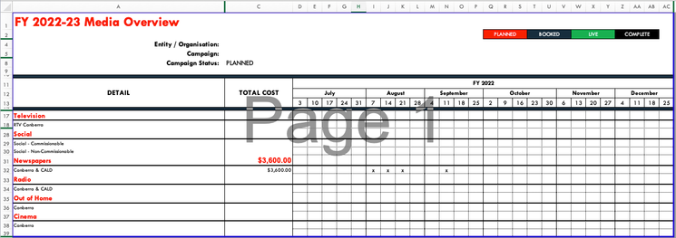
I have a complex Gant chart used for a marketing plan. Each channel (TV ect) connects to a tab and the x's on the page are a formula picking up from another tab when there activity planned for that week. 

I want the x's to highlight different colours pending the campaign status. C8 is where the campaign status is listed and is a drop down list. I want the colour coding to be red if Planned and navy when booked ect. 

My thoughts are to use a formula in conditional formatting to say IF $D$17:$BC$39 has an 'x' AND C8 says PLANNED, turn Red. IF $D$17:$BC$39 has an 'x' AND C8 says BOOKED, turn Blue ect.

Is this even possible? 

 

Thank you very much! 

Sam

[#2 · Accepted solution]

Hi @SamMitchell515 

yes, that's possible:

First, highlight the whole range where the conditional formatting needs to be applied. In my example D17:H19

Then add a rule for every status, like this:

=AND(D17="x";$C$8="Booked")

[#3]

Hi @Martin_Weiss 

Thank you very much for your response. I tried your suggestions it's saying there is a problem with the formula: 

This is what I put in the formula bar:

Am I doing something wrong? 

Thanks
Sam

  

[#4]

Hi @SamMitchell515,

most likely you just need to replace ; with , in your formula. This is due to regional settings (in Germany, we have ; as a separator)

So try :

=AND(D17="x",$C$8="Booked")

instead of

=AND(D17="x";$C$8="Booked")

[#5]

It worked!! Thank you very much Martin, I have been stewing over this forumla for a long time! haha