Conditional formating using a lookup formula.

[Geir Hogstad]

Hi,

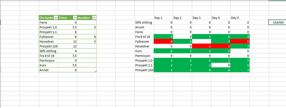
I would like to use condiotional formating to colour an array ie the number ie below the value in a table.

Tried several, but conditional formating using formula does not accept it. Like: 

=XLOOKUP(H5;T_faste[Din kodeliste];T_faste[Number];"")<I5

Colours here is manually adjusted, as an example.

Best Regards

- Geir

[#2 · Accepted solution]

@Geir Hogstad 

Please don't us names (including tables names) In conditional formatting, formula shall be like

=O5<XLOOKUP($H5,$C$5:$C$15,$E$5:$E$15)

[#3]

Thank you @Sergei Baklan It worked perfect. I made it more dynamic using a named range. That worked as well.

Best Regards

- Geir

[#4]

@Geir Hogstad , glad it helped