Conditional Formating Formula

[daniel315]

I have two columns with numbers.

If the number in B column is higher than the number in A column highlight the cell green

If the number in B column is lower than the number in A column highlight the cell red

If the number in B column is within 10% of the number in A column highlight the cell yellow

What formula would you use?

Thank you!

[#2 · Accepted solution]

Hi @daniel315 

you would need 3 rules for conditional formatting:

Yellow: =AND(B1>=A1*0,9;B1<=A1*1,1)

Red:  =B1<A1

Green:  =B1>A1

Depending on your regional settings it might be that you need to replace the first formula like this:

=AND(B1>=A1*0.9,B1<=A1*1.1)

[#3]

Hi @daniel315 

Just about point 3, you mean if B bigger or small than A within %10.

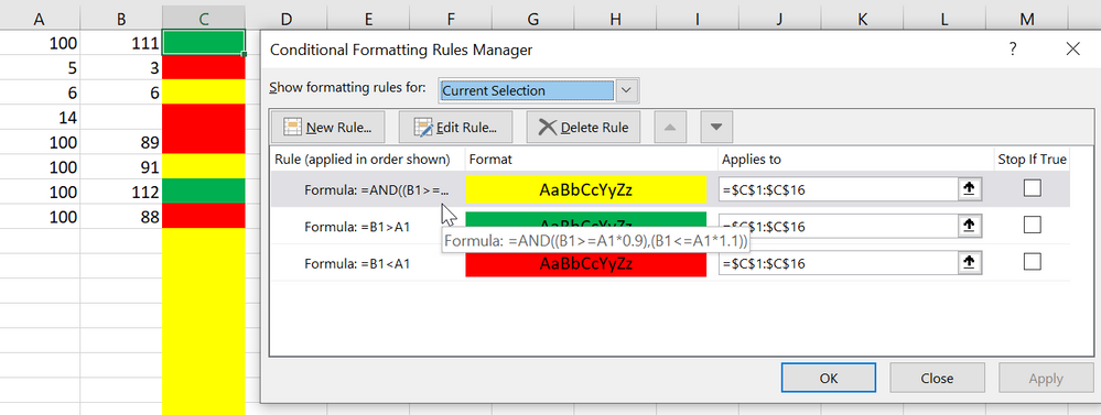
You need to do three rules in the following order, because there will overlap within the %10

=AND((B1>=A1*0.9),(B1<=A1*1.1))        (yellow)

=B1>A1    (green)

=B1<A1    (red)

[#4]

Thank you so much, DTE!

[#5]

Awesome! Thank you so much, Jihad!

[#6]

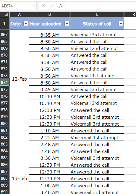
@Martin_Weiss  I could use your expertise with an Excel conditional formatting issue. I want to highlight a row in blue if the value in cell L867 remains "Not contacted yet" for 40 minutes. The L column has a dropdown list, and I'm a bit stuck on the formula. Your assistance would be greatly appreciated.

Thanks a bunch!

[#7]

Hi @Frank1060 

it's not completely clear to me, what the exact rules should be for your formatting. When you say: "not yet contacted" for 40 minutes:

40 minutes related to what exactly? To a certain record in the list? Which one?

I also propose to put your question in a complete new thread, so it gets more attention by other users.

Cheers,

Martin

[#8]

Hi @Martin_Weiss,

When I need to reach out to a candidate, I have 40 minutes to do so. Once I make contact, I update their status from 'Not Contacted Yet' to another one. Now, what I'm looking for is a rule that says if the status doesn't change from 'Not Contacted Yet' within 40 minutes, the entire row should turn blue automatically.

[#9]

Hi @Frank1060 

that's a bit tricky because you need to calculate the time difference between current date/time and the date/time of the call.

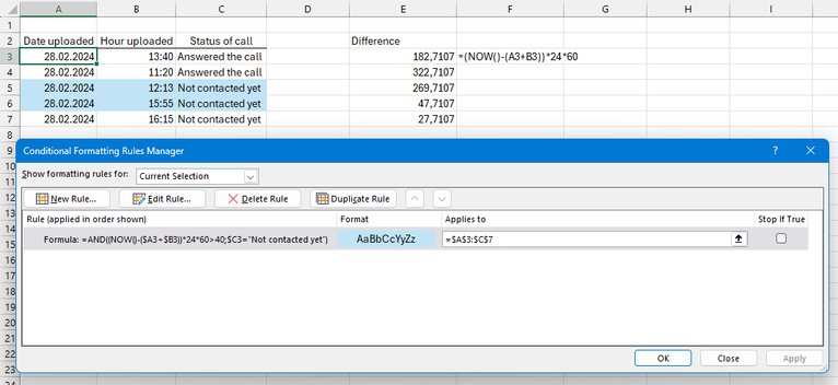
To do this, you need to combine the date and the time of the call (add them up). Then you can calculate the difference to the current time by using the NOW() function.

The formula in the formatting rule would be:

=AND((NOW()-($A3+$B3))*24*60>40;$C3="Not contacted yet")

 

In column E you see the time difference in minutes. This column is not important for the solution, it just illustrates how the formula works.

Hope this helps.

Cheers,
Martin