Conditional Format Formula

[SahuaroCon]

Hello,

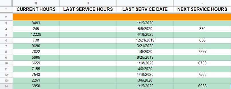
I am trying to set up a formula that highlights an entire row once it meets specifics - which are, if column G # is within 100 of column J # the row is highlighted a light color, and gradually gets dark as the #'s in column G get closer to column J. Shades would get darker in increments of 25, so - Lightest 100>75>50>25>0 Darkest.

I have found formula (=$G3>=$J3) works for if cells in G3 are greater than or equal to J3, but cannot figure out how to do the increments of 25

EX. picture

The rows currently highlighted will be fixed once the rest of the data is entered, but in the example picture, row 4 should be white as is, followed by row 6 which should be the light shade color (G3 is within 100 of J3), followed by row 8 (within 75) > 10 (within 50) > 12 (within 25) > 14 (0) darkest shade.

Thank you

[#2]

@SahuaroCon

I am sure we can support you with this, but I really can't understand what exactly you want there? what do you mean when you say within? try to give us as many details as you can.

cheers

Hemn 

[#3]

@hemnrostam 

My apologies, when I say 'within' I mean..

G3-J3=100 (738-838=100) color shade starts

G8-J8=75 (7822-7897=75)

"

"

"

G14-J14=0 (6958-6958=0)

My company does a service on their machines every 250 hours, the formula I am trying to implement is every time I change #'s in column G (current hours of unit) as it gets closer to column J (up coming service hours). Starting at the 100 marker and gradually getting more and more distinguishable

Hope that makes sense, not very easy to explain

Thank you

[#4]

@SahuaroCon 

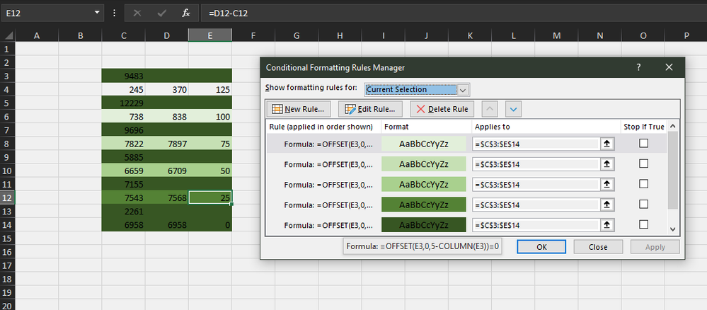
See if this solution points you in the right direction.  Note that I used a different conditional format for each shade your using.  The conditional formulas are identical except for the value of the shade.  For the formula that I've moused over the shade = 0, next one up it = 25, then 50, 75...

Hope this helps!

One more thing to note, you can change the "=0" to ">=0" to catch items that are within a range, in this case 0 up to the value of the previous condition which would be 25.

[#5]

@SahuaroCon  wouldn't it be easier to just add a column "Time Left" and do the conditional formatting on that?  Then you see the remaining hours and you can easily use some nifty built in conditional formatting rules like "Format all cells based on their values" and you can do 2 or 3 color gradients, data bars that fill the cell like a fuel gauge, or icon sets.

@xspJodymaybe I'm missing something but wouldn't you formulas be easier if you just used the '$' to lock the column i.e. =($E3=0)  

[#6]

"Absolutely.  The reason I presented the solution as I did though is because the user did not have a column for this value.  Since I have no way of knowing the full nature behind someones questions I try to present solutions that fit their style as much as I can."

"It may as well still be easier to add a column for this data and refer to it in their conditions as opposed to using the OFFSET function."