- Home
- Microsoft 365
- Excel
- Conditional Format cell color based on value tied to specific value in dropdown list
Conditional Format cell color based on value tied to specific value in dropdown list
- Subscribe to RSS Feed
- Mark Discussion as New
- Mark Discussion as Read
- Pin this Discussion for Current User
- Bookmark
- Subscribe
- Printer Friendly Page
- Mark as New
- Bookmark
- Subscribe
- Mute
- Subscribe to RSS Feed
- Permalink
- Report Inappropriate Content
Jan 21 2020 10:31 AM
Hello,
I looked through a few conditional formatting threads, but did not find my answer. In the sample provided in a second step beyond the indexing i have already done I am trying to tie the month in the drop down list on the sheet labelled "dashboard" with the month and target in the sheet labelled "target" and have the dashboard cells reporting the segments colored Green or Red based on meeting/surpassing or failing to meet the target.
Please respond in a detailed step by step fashion as I am a visual learner :)
- Labels:
-
Excel
-
Formulas and Functions
- Mark as New
- Bookmark
- Subscribe
- Mute
- Subscribe to RSS Feed
- Permalink
- Report Inappropriate Content
Jan 21 2020 12:18 PM
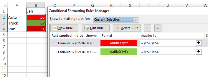
SolutionYou may apply two rules for the range
with formulas
red
=$B2<INDEX(Target!$B$2:$D$13,MATCH($B$1,Target!$A$2:$A$13,0),MATCH($A2,Target!$B$1:$D$1,0))green
=$B2>INDEX(Target!$B$2:$D$13,MATCH($B$1,Target!$A$2:$A$13,0),MATCH($A2,Target!$B$1:$D$1,0))Accepted Solutions
- Mark as New
- Bookmark
- Subscribe
- Mute
- Subscribe to RSS Feed
- Permalink
- Report Inappropriate Content
Jan 21 2020 12:18 PM
SolutionYou may apply two rules for the range
with formulas
red
=$B2<INDEX(Target!$B$2:$D$13,MATCH($B$1,Target!$A$2:$A$13,0),MATCH($A2,Target!$B$1:$D$1,0))green
=$B2>INDEX(Target!$B$2:$D$13,MATCH($B$1,Target!$A$2:$A$13,0),MATCH($A2,Target!$B$1:$D$1,0))