Conditional format a cell that corresponds to todays date

[Sam Collins]

Hi all,

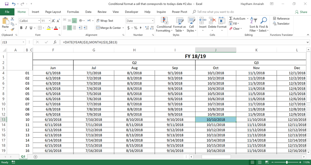
I have a table of sorts with months running across the top and then days running down the left. The months are the first day of each month but formatted to show the just month in "mmm" format e.g. 1/4/18 is Apr.

Down the left is just numbers i.e. 1-31 and formatted as such.

What I want to achieve is a conditional format that highlights the corresponding cell to today's date.

I know it must be some sort of Index Match function to find today's month and the year from the top row and then the day from the numbers on the left, but I just cannot seem to do it.

I have attached the workbook for reference.

Thank you very much
Sam

[#2 · Accepted solution]

Hi Sam,

I've updated the workbook you attached with the below conditional formatting formula to highlight today's date.

=CELL("address",D4)=ADDRESS(DAY(TODAY())+3,CHOOSE(IF(YEAR(TODAY())=2018,1,2),MONTH(TODAY()),MONTH(TODAY())+12),1)

But, please be careful not to change the current layout of the table because the formula depends on it.

Regards,

Haytham

[#3]

Hi Haytham,

Thank you so much - I thought I  had a solution, but it would work when I put it in the Conditional Formatting formula bar. I created this formula that found the correct cell:

=INDEX($D$4:$AA$34, MATCH(DAY(TODAY()), $B$4:$B$34,0), MATCH(DATEVALUE(MONTH(TODAY())&"/"&(YEAR(TODAY()))), $D$3:$AA$3, 0))

Just out of curiosity, how could this be modified to work in the conditional formatting box? If it can at all!

Again, thank you very much for your help!

Sam

[#4]

Thank you.

In fact, I've created a similar formula to this one earlier, but I realized it didn't work!

This is because the INDEX is a lookup function, and it returns the cell's value, not the cell's address which what we need.

To be able to use this formula, you have to fill in all cells with dates, and then adjust the formula in the conditional formatting rule as follows:

=D4=INDEX($D$4:$AA$34, MATCH(DAY(TODAY()), $B$4:$B$34,0), MATCH(DATEVALUE(MONTH(TODAY())&"/"&(YEAR(TODAY()))), $D$3:$AA$3, 0))

This is done in the attached workbook.

Hope that helps

[#5]

I'd suggest

=(D$4+$B4-1)=TODAY()

second sheet attached

[#6]

Hi Haytham,

Thanks for getting back - it does somewhat in that I now understand why Index won't work in a conditional format. However, unfortunately, your suggestion wouldn't work only because I need the cells to be empty as they will be filled in with events etc.

Nonetheless, thank you so much for your help, I think your original formula will work perfectly!

Sam

[#7]

When

=(D$3+ROW()-ROW(D$3))=TODAY()

[#8]

Hi Sam,

I think that the formula suggested by @Sergei Baklan is better and less complicated than my formula.

So I recommend you to use it instead, but with a small correction as follows:

=(D$3+ROW()-4)=TODAY()

Please find it in the attached file

Hope that helps

[#9]

Hi @Haytham Amairah,

You are right, thank you,

=(D$4+ROW()-ROW(D$4)-1)=TODAY()

For the maintenance purposes I'd prefer to keep reference on the row instead of number. If one day you decide to add one more row on the top of the sheet the formula will be adjusted automatically. Otherwise you shall to do that manually.