Concatenate dates

[Ocasio27]

Hello everyone. 

When I try to concatenate 3 columns, one of them has dates, I get in the results column a number that equales a date. Very annoying.

My column formula

=CONCAT([@[Name]],"-",[@[Record _number]],"-",[@[Expiration_Date]])

Example Result:

John Smith-033111-43706

What I really want:

John Smith-033111-08/29/2019

Any help on this? Thanks in advance

[#2]

@Ocasio27 

The best way to achieve your desired outcome is as follows

1. Click anywhere in your data and press CTRL + T. Ensure my data has headers is checked. 

2. Click OK

3. In the Data tab, click on From Table/Range

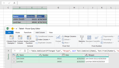
4. In the Power Query editor, select all the three columns 

5. Click on Merge Columns in the Add Column tab

6. In the Merger Column dialogue box, select Custom as Separator

7. In the box below, type in - (as your separator)

8. Click OK

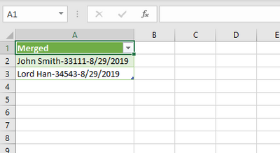
In the caption below, you have the newly added column

9. Right-click on the first 3 columns and select Remove columns

10. Finally, select Close and Load in the Home tab to load the result back to Excel 

That is the final answer.

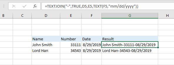
TEXTJOIN method

=TEXTJOIN("-",TRUE,D5,E5,TEXT(F5,"mm/dd/yyyy"))

See attached

If this solve your question, kindly do accept as the Best Response.

Regards

[#3]

@Ocasio27 

Alternatively, try this:

=CONCAT([@Name],"-",[@Record_number],"-",TEXT([@Expiration_Date],"dd/mm/yyyy"))

[#4]

@Ocasio27 

In addition, you can use flash fill (programming by example)

1. Type in the values in each of the three columns and separate with - 

2. Click Enter

3. Execute CTRL + 3.

This is much faster

[#5]

@Riny_van_Eekelen 

=CONCAT([@Name],"-",[@Record_number],"-",TEXT([@Expiration_Date],"dd/mm/yyyy"))

=CONCAT([@[Name]],"-",[@Record_number],"-",TEXT([@[Expiration_Date]],"dd/mm/yyyy"))

Made a slight modification. For some reason I MUST keep the first and last columns with [@[]] or else i get a mess, IDK why

[#6]

@Ocasio27 

What's "IDK"?

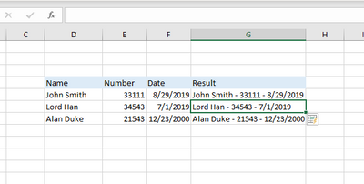
I replicated your example as shown in the picture below. Don't understand why you must have the extra

"[@[]]". But if it works for you, that's okay, I guess.

[#7]

@Riny_van_Eekelen 

 
I mean I dont know

My formula bar will automatically add those []. Even if i try to change the whole formula by adding the table as reference it turns it back to those extra []. In the end, it works anyway so OK

[#8]

@Ocasio27 

That's how structured references work, you may check more here Using structured references with Excel tables 

[#9]

@Ocasio27 

I am now trying to do this in a Power Pivot table, it does not accept more than 2 arguments. How can I do this in power pivot.

[#10 · Accepted solution]

@Ocasio27 

In DAX

you may use

=CONCATENATE(Table1[Name],CONCATENATE("-",CONCATENATE(Table1[Record Number],CONCATENATE("-",Table1[Expiration Date]))))

but much better is

=Table1[Name] & "-" & Table1[Record Number] & "-" & Table1[Expiration Date]