Complicated formula, need some help!

[AustinFindley]

I am trying to come up with a formula using conditional formatting that will highlight an individuals name green if the person has met certain requirements. I understand the logic of what I am trying to do, but I don’t speak the language well enough!

If you haven’t served in the military and need to get familiar with some of the Jargon that Im dealing with, here is some key info-

SPC and CPL are the same pay grade and Promote to SGT
SGT SZ means Secondary Zone promotion from SPC or CPL to SGT. This is an earlier promotion than SGT PZ (Primary Zone)
The Primary zone will have greater than or equal to points to the secondary zone (but never less than).

SGT is the rank above SPC or CPL and Promoted to SSG. SSG SZ and SSG PZ are the same concept as above but one pay grade higher.

Im order for a Soldier to promote, the need a certain amount of points based on several variables that add to the total points. My actual spreadsheet has each section broken down and added up to make the total.

My goal is to simply create a comparison based on True and False. I attached a sample spreadsheet that has some prefilled cells to match my logic here-
IF NAME is a SPC OR CPL AND has TOTAL POINTS GREATER THAN OR EQUAL TO SGT SZ highlight his name in a Green fill

IF NAME is a SGT and has greater than or equal total points to SSG SZ highlight his name green.

I hope this makes sense, How do I format that?

[#2]

@AustinFindley 

Conditional formatting rule formula applied to that range

could be

=( ($B2="SPC") + ($B2="CPL") )*($D2>=$B$11) + ( $B2="SGT" )*( $D2>=$D$11 )

Just in case, multiplication means logical AND, summation logical OR

[#3]

Thank you, I apologize for not getting back sooner. I’ve been out of the office. I forgot to mention in my original post that the other criteria that has to be met is that the individuals “MOS” has to match the MOS for the required points. So in my example there are 35M and 35N both of these MOS will have different varying promotion points from month to month.

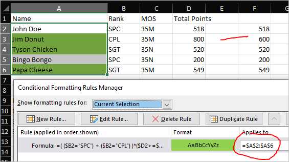
How would I go about adding that condition into the true/false?

CPL Jim Donut is a 35M with 800 points and so meets the point requirements and is highlighted green.

SPC Bingo Bongo only has 200 points and does not meet his requirements and is highlighted orange.

[#4]

@AustinFindley 

That could be

=( ($B2="SPC") + ($B2="CPL") )*($D2>= LOOKUP($C2,$A$11:$A$12,$B$11:$B$12)  ) + ( $B2="SGT" )*( $D2>=  LOOKUP($C2,$A$11:$A$12,$D$11:$D$12) )

[#5 · Accepted solution]

@AustinFindley 

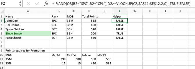
If I were you, I'd create what's called a "helper column" to do the testing, produce a TRUE or FALSE result, and use that as the basis for the conditional formatting, rather than building all of the logic into the formula in the conditional formatting dialog box. It is possible, as Sergei has demonstrated, to build it all into the Conditional Formatting rule, but those are tricky enough to begin with.

In your case, you might even create two or more helper columns, one to test for current position qualification, another to test for sufficient points, and then a third that nets out the result and serves as the basis for the conditional format color.

Using helper columns is a way of making the logic more visible, highlighting where the discrepancy might exist (or an error: somebody you know qualifies yet isn't turning up). It's a truism in computer history--spreadsheet history--that we can start trusting the results ("It's what the computer is telling us!") when in fact there's a subtle error embedded somewhere in a formula. So visibility of the variables, the assumptions, the tests, isn't a bad thing. Once you're confident, having truly tested it, you can hide the helper columns yet still have them there.

So in the attached I created a single helper column to illustrate the process. I may have misunderstood your criteria, but it still can illustrate the process.

[#6]

Thank you, this is a good idea. I tried Mr Baklans solution, but I feel that when I move that logic to my main spreadsheet, I will undoubtably mess it up. But still, thank you Mr. Balkan for the work because I know understand the HOW and WHY for what I can doing.

And Mathetes, thank you for that outside the box idea. Because there are actually several more less complicated variables to what I am working on, I think these helper columns will allow me to compartmentalism the different variables and simplify the data.

[#7]

This works well, but I am not confident in my ability to reproduce the results effectively in my larger spreadsheet! Thank you for your answers, it taught me the primary info that I was looking for! You are an absolute Excel wizard.