Comparing Two Worksheets, please help!

[surefirewizard]

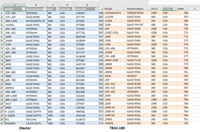
 I have two worksheets in a workbook, 'Master' and 'TB43-180'.  I need something that will check each line in the Master against each line in TB43-180, such that if the model, nomenclature, and Syscode match but the INTVL doesn't it will say FALSE.  In other words, if all four match it is TRUE but if the INTVL does not it is FALSE.  It is guaranteed that model, nomenclature, and Syscode will match because the Master spreadsheet is, in essence, derived from TB43-180.  What I am looking for is where the INTVL doesn't match when compared to TB43-180 because those are the records I will need to change.  I envision a formula or whatever that I can put into a column in the Master and just drag it down to populate.  Pretty sure this will involve INDEX, IF, and ANDs but I just don't have a grasp on it.  Thank you all! 

[#2]

Hi.
Given both sheets have identical structure, field and cell data and formatting, and line ordering, I'd try the 1st of the following options, but the 2nd may be just useful as well in case the differences between both spreadsheets is expected to be minimal.

1. Create a new sheet in your file or a new book in case you don't want to touch your source data file, and put in A1 a comparison between each A1 cell from both Master and TB43-180.
eg.: Cell A1: ='[YourFile.xlsx]Master'!$A$1='[YourFile.xlsx]TB43-180'!$A$1
And copy it to the right and bottom to the extent of both tables.
You will get a TRUE/FALSE as result for each corresponding cell. For easier spotting of FALSES you can apply conditional formatting to the entire range with 'red' for FALSES or the like.

2. Another possibility is to export both sheets as csv files and just compare them with a text comparison program (WinMerge is a nice and free opensource alternative). It will highlight every line and differing data between both csv files.

Hope this helps. Please note both solutions are intended to be simple. It can be done with more elaborate programming or more complex formulas, but given the case, it may not be deemed necessary.

[#3]

@surefirewizard Perhaps the easiest method to follow would be to add a column to each table where you concatenate the four relevant columns. Then in the second table, add yet another column where you VLOOKUP (or XLOOKUP if your Excel version supports it) the concatenated values from Table2 in the added column in Table1. Anything other than #NA means that a matching value was found. #NA is thus equivalent to FALSE in your example.

But, if these are very large tables and you have to this on a regular basis, I would use Power Query.

[#4]

Looking more closely at your picture, my best advice is to prepare an "index" column by concatenating 2 or more "key" fields (columns) in each table and then perform a VLOOKUP, comparing the values returned for each record (line) matching the "key"
eg.: [Model]&[Barcode] to get a unique line ID and then use this value as search value in VLOOKUP.

[#5]

Villaseca, thank you for your help but I honestly would not have a clue how to do that. Would you be able to show me what code is needed and where based on the worksheets I provided?

[#6]

@surefirewizard 

It looks like you have structured tables in two sheets

You may add to Master another column (Test) with formula in it like

=IF( ISNA(
          XMATCH( [@Model]&[@Nomenclature]&[@Syscode]&[@Intvl],
                   TB43_180[Model]&TB43_180[Nomenclature]&TB43_180[Syscode]&TB43_180[Intvl]) ),
      "not match", "" )

and apply conditional formatting to highlight not matched records.

Similar could be done with ranges and MATCH().

[#7]

@Sergei Baklan Thanks, figured it out on my own but your solution is much more elegant!

[#8]

Also, I don't have XMATCH on my version of Excel. Can you provide the code with ranges and MATCH?

[#9]

@surefirewizard 

With MATCH() just add to it third parameter as zero:

=IF( ISNA(
          MATCH( [@Model]&[@Nomenclature]&[@Syscode]&[@Intvl],
                  TB43_180[Model] &
                  TB43_180[Nomenclature] &
                  TB43_180[Syscode] &
                  TB43_180[Intvl],
                  0 ) ),
      "not match", "" )

I'm almost sure you have structured tables. But if ranges it depends on how data is structured exactly, plus it'll be better to use dynamic range. In simple case with hardcoding ranges

=IF( ISNA(
          MATCH( $C3 & $D3 & $E3 & $F3,
                 'TB43-180'!$B$5:$B$16 &
                 'TB43-180'!$C$5:$C$16 &
                 'TB43-180'!$D$5:$D$16 &
                 'TB43-180'!$E$5:$E$16,
                  0 ) ),
      "not match", "" )

and drag or Ctrl+D such cell down.