Comparing data in columns on 2 separate worksheets

[Jeri_info4u]

Good afternoon,

I am currently running Windows 10 and I am using 

Microsoft® Excel® for Microsoft 365 MSO (Version 2110 Build 16.0.14527.20234) 32-bit.

I am looking for a daily report that lets me compare the number of QA calls scored from the platform we use to score calls (Raw Data) and the number of calls scored submitted to Smartsheets (data input by the scoring user). The numbers from both don’t always match and we’re trying to figure out why. Ideally, we’d like a big picture view as well as being able to see it broken out by QA Specialist (scoring user).

Oftentimes, these numbers do not match as one is raw data and the other is input by the agent and I need to determine where the discrepancies lie between the two forms of data.

First and foremost, I need to compare the number of calls graded each day with the report from Smartsheets and the raw data from the platform used. Essentially, the goal is to determine what numbers don't match and why per agent by date. For now, I would like to start with 11/22/21 - 11/25/21, as it seems that would be easiest when trying to determine the best avenue to take. Then I will look at it daily and then monthly, etc. 

I have attached an Excel Workbook with two worksheets. Each worksheet is labeled. The first worksheet is called Smartsheets Data (Spec Input) and the second worksheet is called QA Raw Data Platform. As it sounds, the Smartsheets is information regarding a scored call input into a SmartSheets form that includes the date the call was scored and the agent who scored the call. The QA Raw Data Platform is pulled from a report done on the platform used to score calls and it, too, includes the date the call was scored and the agent who scored the call. 

I need the best formula or method to use to calculate the number of calls scored by each agent by date on the Smartsheets form and then I need to do that same calculation for the QA Raw Data Platform sheet. After the calculations are one, I need to compare the data from Smartsheets with the data from the QA Raw Data Platform and see which agent has numbers that do not match and which day do the numbers not match. For example, let's say that the Smartsheets Data report shows Sofia graded 27 calls for the week of 11/22/21 - 11/25/21 and the QA Raw Data report shows Sofia only graded 23 calls for the week of 11/22/21 - 11/25/21. I need another formula or method in place that compares the total number of graded calls per day for Sofia for the specified week on sheet one and sheet two so that it shows which days have the discrepancies.  

I just need the quickest and most efficient way to have the totals for calls scored per agent per the date on each sheet. Then I need to be able to compare those totals from both sheets that will show which days do not have matching numbers and for which agent.

Any and all help is greatly appreciated and the sooner the better so I can submit this report.

Thank you so much! 

[#2]

@Jeri_info4u I would create on list and add an extra column containing the source of the data. Then you can create a pivot table and summarise everything in one pivot table. The attached file contains such a "quick-and-dirty" pivot table.

[#3]

@Riny_van_Eekelen Thank you for the response! I was able to create the pivot table and get the desired results using your method. There's one exception. How did you get the calculations in red on the Smartsheets data to produce? My Pivot Table looks just like yours minus the red calculations.

[#4]

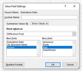
@Jeri_info4u Omitted to mention the variance columns. I added another value field for "Evaluation Date" and set it to 'Show Value As' difference from Raw.

That will produce some extra columns with pretty ugly and long headers, which I just replace with a single space. In the Raw group, the variances will obviously be blank (note I reduced the column width considerably), but in the SmartSheets group you will get some variances. Custom formatted these with  0;-0; (this will suppress any zeroes) and colored them red to make them stand out. 

[#5]

@Riny_van_Eekelen Thanks again for your response! I must not be doing something right. I am doing it in such a way that it matches your screenshot but I keep getting the error message that I cannot enter a null value as an item or field name in a pivot table report. I am not sure where to put the 0;-0; or how to add the variance as you did.

[#6]

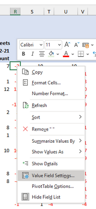
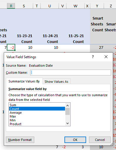
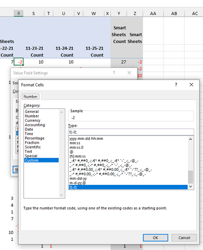
@Jeri_info4u The custom formatting is entered in the following steps.

Select any cell in the variance column, right-click,

select Value Field Settings...

Press the Number Format button (bottom left)

Choose custom and enter the required format in the Type-field. Press OK.

Don't really understand why you get a "null value" error message. Can you otherwise upload your file? Then I can have a look.

[#7]

I am so sorry I am just now getting back to you but I have been super busy and had to work a lot of overtime during the holiday. I am going to upload what my file looks like. I'm obviously missing a step somewhere because I am not getting a variance column to produce. Allow me a moment to upload that data.