Comparing Data from Two Excels - Most Views One & Most Engagements

[Paul_PP]

I have two excel sheets.

One, I've sorted by "most engagements" and the other sorted by "most views."

Each sheet has the same emails for each employee.

I'd like to compare data from the two sheets together and find out from the individuals with the "most views" who from that list has the "most engagements."

Could folks recommend the best way. 

I assume what way could be combine data using the pivot table with the emails as the common denominator and match engagements to the "views" list by email. 

Then sort first by "views" then "engagements".

If that's the best way, could someone share the easy-to-follow instructions for pivot tables?

Thanks

[#2]

You could do an xlookup here, using the employee email, on the Most Views sheet, look up the number of engagements for that same email on your engagements sheet. This will list out engagements along side views so you can have views and engagements side by side. Then use a "Custom sort" with two levels, to sort first by views then engagements.

Let me know if you need a more in depth explanation!

[#3]

@DKoontz Thanks for pointing me in the right direction.

As I'm a newbie with , if you could provide me with a more in-depth explanation, I'd be most grateful.

[#4]

@Paul_PP 

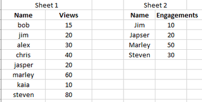
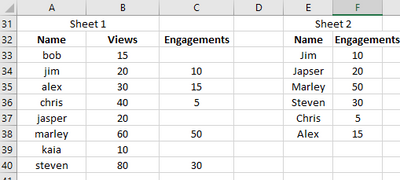
I'll use two lists side by side so it'll be easier to show, but this will work across sheets too. So I would combine your two data lists using a look up, starting with this (your two sheets):

xlookup in column C  =+XLOOKUP(A33,E:E,F:F,"")  this transfers engagements from sheet 2, no matter what the order, and matches to the correct person or email in your case.

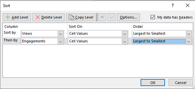
Select your data on sheet one and custom Sort:

Then add two sort by levels, first by views largest to smallest, then engagements largest to smallest:

[#5]

@DKoontz 

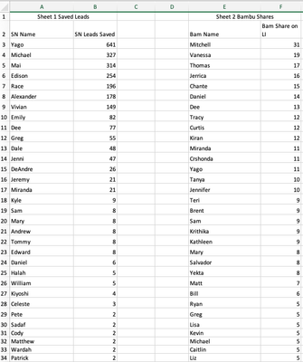
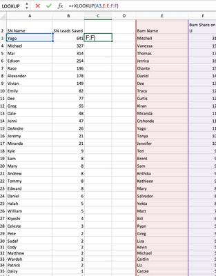
I'm able to partially set up the LOOKUP, but I can get the formula to go through. I set up the sheet like this, but keep getting a "#NAME?"

 Then I've tried multiple formulaS in C3 for the column C: "=Xlookup(A3,E3:E35,F3:F35)" ; =+LOOKUP(A3,E:E,F:F) . Nothing is working. Can you tell where I'm missing something?

 

[#6]

@Paul_PP 

As a comment, discussion could much more efficient if share sample file, not screenshots. "Nothing is working" is too abstract. Screenshot says only that XLOOKUP() is available in your environment. But returns result which you don't expect, and from screenshot is not clear which one. #NAME! error could be caused by few reasons, without the file it's long discussion to understand by which one exactly. 

[#7]

@Sergei Baklan 

I know XLOOKUP works with the web version of Excel, as for desktop versions, I think it is available from Office 2019 onwards.

The alternative is VLOOKUP, Syntax: VLOOKUP(<value to lookup>, <range of data with lookup field on the left of the range>, <column number to of the range to return>, FALSE).  The lookup value must be in the first column of the range.

Example based on your data:

	A	B	D	E	F
1	SN Name	SN Leads Saved		SN Name	Result
2	Yago	641		Mal	314
3	Michael	327
4	Mal	314

In the example above, the cell in F2 has =VLOOKUP(E2,A2:B4,2,FALSE).  A2:B4 is the range to look up the value with 2 being the 2nd column of the range.  The False on the end dictates if you want an exact value or the closest match (False = Exact Match, True = Closest Match)

[#8]

@Mathew_Vaughan 

Nope, it's not on 2019. Supported version are mentioned here XLOOKUP function - Office Support (microsoft.com)

IMHO, much better alternative for XLOOKUP is INDEX/MATCH.

[#9]

Thanks, I can confirm it's only available on web-based platforms (including iPad, Android). Been using tablets for too long.

[#10]

Index/Match is a bit less intuitive, especially if you aren't familiar with how lookups work.

[#11]

@DKoontz 

True. I only would like to say that XLOOKUP was designed to take power of INDEX/MATCH in more intuitive form.

[#12]

Thanks @Sergei Baklan for the prompt. Here's the data. I appreciate you and @DKoontz looking at this.

[#13]

No problem! I see where the mistake was, in your formula you have =+Xlookup(A3,E:E:F:F), it should be =+Xlookup(A3,E:E,F:F), you had an extra : where it should have been a comma. If you fill down this formula, it'll bring over all of the shares for each person. Where it returns an #N/A, that person isn't represented in column E, the share data set.

[#14]

To add to this, =+XLOOKUP(A3,E:E,F:F,0), the extra 0, will return 0 if not found instead of #N/A. Which may be helpful

[#15]

@DKoontz It still does not seem to be working. I'm using Excel 2016, so could that be at play?

[#16]

@Paul_PP 

Excel 2016 doesn't support XLOOKUP(). Formula like this could work

=IFNA(
  INDEX($F3:INDEX($F$3:$F$10000,COUNTA($E$3:$E$10000)),
        MATCH($A3, $E3:INDEX($E$3:$E$10000,COUNTA($E$3:$E$10000)), 0)),
 "no match")

Please check attached.