Compare Two Columns

[pbexpresss]

I have a list of employees who submitted their daily reports.  I need to compare this list with the complete employee roster to determine which employees did not submit their daily report.  How can I do that?

[#2]

@pbexpresss 

you forgot to mention which worksheet you would like the result

[#3]

@pbexpresss 

It depends on which version of Excel you are, how your data is organized and in which form you'd like to see the result.

That could be helper COUNTIF() column with filtering on it, could be dynamic arrays formulae, could be conditional formatting, could be Power Query, whatever.

[#4]

Okay. Here are the details. Each day my employees submit a daily report to the cloud. A summary report is run automatically and emailed to me by the software company. I need to create a list at the bottom of the report of names of employees who did not submit a report. I was trying to compare this report with a master file of names. How should I do this?

[#5]

@pbexpresss 

Thank you, but still better to have sample file.

If these are two different file you may use Power Query to compare data an return the table with records which don't meet condition.

[#6]

I will give Power Query a try.

Thanks

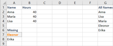
[#7 · Accepted solution]

@pbexpresss Hi. Assuming Excel 365, this is a way

XMATCH looks for all names among those reported.

ISERROR becomes true if they are not in the list of reported hours

FILTER shows all names that have not reported

=FILTER(G2:G6;ISERROR(XMATCH(G2:G6;A2:A4)))

Change G2:G6 to range in your workbook with all names.

Using the function LET makes it easier to read and test the different parts.

Last line is what the cell outputs and changing "output" to eg haveReport shows that part of the calculation.

I prefer to have the definitions indented.

=LET(allNames;G2:G6;
         reportedNames;A2:A4;
haveReported;XMATCH(allNames;reportedNames);
haveNotReported;ISERROR(haveReported);
output;FILTER(allNames;haveNotReported);
output
)

[#8]

@bosinander The combination of functions worked perfectly.  I created a file that maintains my master employee list.  When I retrieve the file summarizing my employees' daily report submissions, the macro I created uses your suggestions to compare the list from one file with the other file. Then it gives me a list of employees who did not work that day at the bottom of the daily report submission report.

Thanks,

[#9]

=FILTER(G2:G6,ISERROR(XMATCH(G2:G6,A2:A4)))
thx for the answer, it was usfull for me as well, however if you want to copy &past do it from my post
since in the original answer, there is an error they put an ";" instead " ,"

[#10]

Yes, the local settings on my computer uses semicolon instead of comma.
Opening the attached file though would adapt to your local settings as well as translated function names depending on your chosen language.
Thanks for the note :)