Compare two columns and highlight matches

[Assino960]

Hello everyone

i'm searching how to Compare two columns and highlight matches (1 on 1)
there is many different ways but what i want is to highlight one cell if there is only 1 cell that contains the same value on the other column
for example :

with the methods i use the "126" value highlighted twice in the first column even that there is one in the second one

and what i want :

i hope i've explained it well :) .

[#2]

Hi @Assino960 

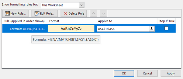
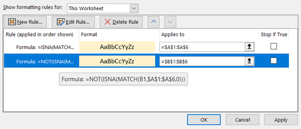
Please find below the logic which you need to paste the conditional formatting using formula

make sure you select the range correctly. I'm attaching the sample sheet for your ready reference.

 

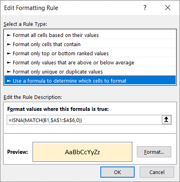
Logic 01

=ISNA(MATCH(B1,$A$1:$A$6,0))

 

Logic 02

=NOT(ISNA(MATCH(B1,$A$1:$A$6,0)))

Regards, Faraz Shaikh | MCT, MIE, MOS Master, Excel Expert

If you find the above solution resolved your query don't forget mark as Official/Best Answer to help the other members find it more

[#3]

@Assino960 

You can do this with conditional formatting.

Insert a row above the data to make it easier.

Select A2:A7.

On the Home tab of the ribbon, select Conditional Formatting > New Rule...

Select 'Use a formula to determine which cells to format'.

Enter the formula

=AND(ISNUMBER(MATCH(A2,$B$2:$B$7,0)),COUNTIF(A$1:A1,A2)=0)

Click Format...

Specify the desired font color and/or fill color.

Click OK, then click OK again.

Do the same for B2:B7, but with the formula

=AND(ISNUMBER(MATCH(B2,$A$2:$A$7,0)),COUNTIF(B$1:B1,B2)=0)

[#4]

@Faraz Shaikh 

Hi.
thanks for replying :)
i appreciate your help

But when i use your method on a large data i don't get the result i want, 

what i want as result that the sum of highlighted cells in A = to the highlighted cells in B

(if there is 2 cells that contains "x" in column 1, and 3 "x" in column 2, i  want to highlight two cells in each column).

[#5]

@Hans Vogelaar 

Hi.
thanks for replying:)
i appreciate your help

But when i use your method on a large data i don't get the result i want, and also tehere is a lot of matches that are not highlighted.

what i want as result that the sum of highlighted cells in A = to the highlighted cells in B

(if there is 2 cells that contains "x" in column 1, and 3 "x" in column 2, i  want to highlight two cells in each column).

[#6 · Accepted solution]

@Assino960  well you changed the rules a little. lol.  As for the errors in @Hans Vogelaar method that was because you had an error in the formula in that sheet.  You probably shifted the sheet / target range because instead of A$1:A1 you had A$2:A2 and instead of referencing A2 it was looking at A3, which is what threw everything off.  That all said I think this set of conditional formatting formulas might be what you want:

=COUNTIF(A$2:A2,A2)<=COUNTIF(B:B,A2)

=COUNTIF(B$2:B2,B2)<=COUNTIF(A:A,B2)

see attached sheet.

[#7]

Hi,

thanks all of you for helping me out I really appreciate it :).