combining sumifs and sumproduct

[jomynitima]

I need to calculate 2 columns in a table, with specific criteria, mentioned in a other column of the same table

=SUMIFS(SUMPRODUCT(Table4[Sales price
per unit];Table4[Earchair]);"Table4[Calc
group]";M9#)

It's should be dynamic too

Thanks for any help

[#2]

@jomynitima 

Let forget your formula for a while, what exactly you'd like to calculate for each Calc group listed in M4# spill?

[#3]

@Sergei Baklan 

In N9 I need to show how much fabric costs there is the product EARCHAIR (column Earchair, is written how much of the material (tabel Row, criteria CALC Group) is used in this product)

[#4]

Hello @Sergei Baklan,

What would be the correct formula to calculate 2 columns in a tabel, with criteria's.

I am new here and would know how to find these kind of answers

[#5]

@Sergei Baklan 

First of all, a happy New Year!
I am still puzzling, hope you can help

In a table are specified in rows of materials, which at the end of this dynamic table are filled in in product columns with numbers.
In another sheet the price of these products has to be calculated grouped for steel, wood, working time...
I would like to use a validation to select products from the table headers, so that I can compare prices.

Any help would be great.

[#6]

@jomynitima 

Happy New Year!

Sorry, but I missed with your description. Could you please specify the same but more close to Excel file terms. 

table are specified in rows of materials - is that Table16?

end of this dynamic table - same table or another one?

In another sheet the price.. - is that DT sheet?

etc.

I'm not familiar with your business and your project and don't remember what we discussed previous time, sorry for that. Please give more straightforward explanation what, where and base on what it shall be calculated.

Thank you for understanding.

[#7]

@Sergei Baklan 

apologies for my brief and incomplete explanation

Yes, in Table16 are all the material specs (Column A:L), starting from Column M, I am putting all amounts off materials that goes into the Products (Table-Headers).  These need to be calculated in DT!D9

I need to calculated SELLING PRICES * the amounts specified in MinMat!Column M

In TabDT D3:G3 is a criteria of the products that can choose to be calculated into the material groups sorted in C9 (also from Table16) starting in Cell D9

I hope this explains a little better what I need

[#8]

@jomynitima 

Thank you. I'll check bit later tonight what I can do, explanation looks understandable (for me of course) now.

[#9 · Accepted solution]

@jomynitima 

I guess you are on DA Excel, thus have XLOOKUP(). Formula in D9 could be

=SUMPRODUCT(IFERROR(XLOOKUP(D$3,Tabel16[#Headers],Tabel16[#Data])*1,0)*Tabel16[[Selling
in euro
Price]:[Selling
in euro
Price]]*(Tabel16[[Material
group]:[Material
group]]=$C9))*(1+$C$5+$C$6)

and drag it down and to the right. I wrap first XLOOKUP with IFERROR since you have texts in some cells (actually spaces), such values are considered as zeroes.

[#10]

@Sergei Baklan 

Thanks so much, after I translated to English formulas to Dutch it works perfectly.  Now I just have to study it so I understand what I did wrong all this time.

The only strange thing is that I cannot drag the formula. Probably an MS Insider (fast) bug they need to repair.  If the formula is in the formula-bar in 1 line it doesn't work and if it's in more lines it works!!? (screenshots).

[#11]

@jomynitima 

Without the file it's bit hard to say what are the issues. In general

- you don't need to translate formulas manually. If you open the file attached to my previous post, formula automatically appears in your locale. In addition, you may use this great tool https://en.excel-translator.de/translator/

- there is absolutely no difference in behavior of multi-line formula and one compacted into one line. Of course, if the latest done correctly. That includes ability to drag cell with formula.

[#12]

@Sergei Baklan 

Thanks again Sergei

I added the file that I typed in the translated formula, for you to have a look at.

Hope you find something wrong in it.

Have a nice weekend

[#13]

@jomynitima 

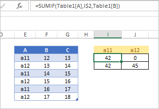
You didn't fixed references on columns in Table16 within the formula. Let me explain on the sample. For such data

in I3 we SUMIF table based on criteria in I2:

=SUMIF(Table1[A],I$2,Table1[B])

If we now drag I3 to the right on J3 formula will be automatically converted to

=SUMIF(Table1[B],J$2,Table1[C])

- it takes next columns in the table since in formula we have kind of relative references. Thus we have wrong result.

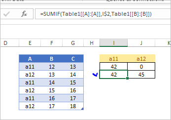
To fix columns with structured references we shall use

=SUMIF(Table1[[A]:[A]],I$2,Table1[[B]:[B]])

as in I4:

If we drag this formula to the right on J4 we have correct references on table columns and correct result:

=SUMIF(Table1[[A]:[A]],J$2,Table1[[B]:[B]])

I corrected formula in your file as explained above

=SUMPRODUCT(IFERROR(XLOOKUP(D$3,Tabel16[#Headers],Tabel16)*1,0)*Tabel16[[Selling
in euro
Price]:[Selling
in euro
Price]]*(Tabel16[[Material
group]:[Material
group]]=$C9))*(1+$C$5+$C$6)

with dragging it returned result is correct. Please note, above formula is actually single line one (i.e. I didn't add line break manually), we have it as multi-line since texts in columns names include line breaks.

If we add line breaks manually (second column), like

=SUMPRODUCT(
   IFERROR(
      XLOOKUP(
         E$3,
         Tabel16[#Headers],Tabel16
      )*1,0
   ) * Tabel16[[Selling
in euro
Price]:[Selling
in euro
Price]] *
   (Tabel16[[Material
group]:[Material
group]]=$C9)
   ) *
(1+$C$5+$C$6)

nothing changes in behavior. The only don't touch column names, they shall be as they are.

Both files are attached.