Combine/Rearrange Rows and Columns

[Rob Nunley]

Hi,

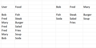
I am trying to combine and rearrange two columns of data into a different format.  Would like the User column to become the header and the Food column to populate under the corresponding user.  I've tried using the Transpose function but have not gotten it to work. I've attached a picture of the original data and the results.   

Thanks!

 

[#2 · Accepted solution]

@Rob Nunley 

For such layout

if you are on Excel with Dynamic Array that could be

in E2

=TRANSPOSE(UNIQUE(B3:B9))

in E3

=FILTER($C$3:$C$9,$B$3:$B$9=E$2)

and drag to the right.

Another option with more traditional functions

In I2

=IFERROR(INDEX($B$3:$B$9,AGGREGATE(15,6,1/(COUNTIF($H$2:H2,$B$3:$B$9)=0)*(ROW($B$3:$B$9)-ROW($B$2)),1)),"")

in I3

=IFERROR(INDEX($C$3:$C$9,AGGREGATE(15,6,1/(COUNTIF(I$2:I2,$C$3:$C$9)=0)/($B$3:$B$9=I$2)*(ROW($C$3:$C$9)-ROW($C$2)),1)),"")

and drag to the right and down.

Power Query also could be an option.

[#3]

@Rob Nunley 

Just in case, added Power Query

Generated script:

let
    Source = Excel.CurrentWorkbook(),
    SelectRange = Table.SelectRows(Source, each ([Name] = "Range")),
    GetRange = SelectRange{[Name="Range"]}[Content],
    AddHeaders = Table.PromoteHeaders(
        GetRange,
        [PromoteAllScalars=true]
    ),
    GroupByFirstColumn = Table.Group(
        AddHeaders,
        {"U"},
        {{"AllRows", each _[F]}}
    ),
    FinalTable = Table.FromColumns(
        GroupByFirstColumn[AllRows],
        GroupByFirstColumn[U]
    )
in
    FinalTable

[#4]

Thanks @Sergei Baklan, 

My workbook has a few worksheets.  This data is pulled from a worksheet that is a subset of the whole data set via a filter.  Is there a way for this formula only pull data from that filtered subset of the data?

[#5]

@Rob Nunley 

On filtered content these are other functions, see for example https://www.get-digital-help.com/extract-unique-distinct-values-from-a-filtered-table-udf-and-array-...