Cell data based on input lists from multiple columns

[Cliff_P]

It's been several years since I've been an excel junky, so I'm hoping the subject even makes sense.

I have a pricing sheet I am working on, that uses lists for in-cell dropdown selection. I was considering IFS (AND) nested statement, but it will likely end up extremely complicated and long for what I want to achieve.

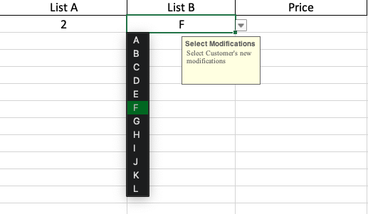
Sheet A, I have 3 columns. 1 and 2 are the list drop down, and 3 is the output based on the selection from 1 and 2.

Sheet B contains the data for columns 1, 2 and 3. Column 3 in sheet B does not correlate directly to column 1 and 2 (A1 and B1 =/= C1, but could equal C5).

If I'm going about this the wrong way, I'm all ears.

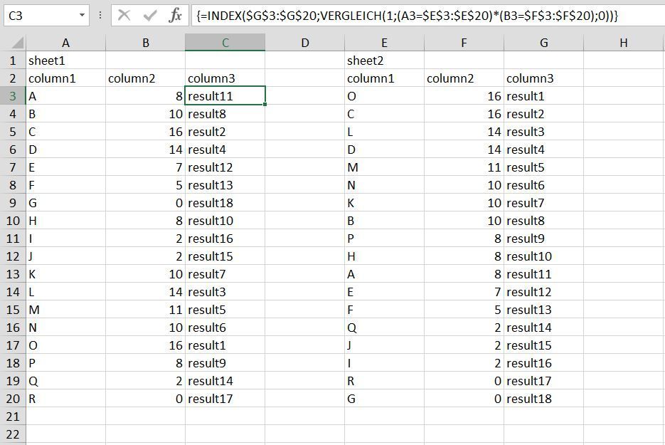
[#2 · Accepted solution]

@Cliff_P 

=INDEX($G$3:$G$20,MATCH(1,(A3=$E$3:$E$20)*(B3=$F$3:$F$20),0))

Maybe with INDEX and MATCH. Enter the formula with ctrl+shift+enter if you don't work with Office365 or 2021. The formula can be adapted as required.

[#3]

@OliverScheurich 

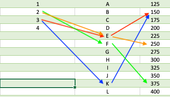
I think maybe my brain wasn't able to accurately depict what I meant, so I've attached two images. First depicts the list data on the second sheet. A3 and B5 for example have a cost of $150. A3 and B11 however also have a cost of $150. A2 and B6 would have a cost of $375,  A2 and B5 would be $250.

Based on your screenshot and formula in your response, it seems to follow fixed and not variable outputs?

[#4]

@Cliff_P 

Does variable output mean that e.g. A3 and B5 can have cost of $150 today and $320 next week? Or is the cost for e.g. A3 and B5 always the (variable) value in D2?

The suggested formula follows fixed input and output criteria which can be used in an IF or IFS statement. With INDEX and MATCH you can reference very large datasets whereas IF and IFS are restricted to a certain number of nestings.

You were considering IFS (AND) nested statement, but it would likely end up extremely complicated and long. What would be the "Something is true1" and "Value if true1" and the "Something is true2" and "Value if true2" and so on conditions in your IFS formula? From your example i don't understand why A3 and B5 for example have a cost of $150 and i wonder what the cost for A4 and B8 would be. Which rule can be applied to return the cost for any combination?

[#5]

@OliverScheurich 

After reading your response a few times, I think I pretty much sorted this out, and your initial solution will work for what I need. I was over-complicating things for the sake of making it easy for my staff to use the sheet. The price of the A3 and B5 will not change on the data side of things.  I will work on making this simple for my sake, and the sake of the people that will be using the sheet. Thanks!