- Home
- Microsoft 365
- Excel
- Cannot group that selection in a pivot table
Cannot group that selection in a pivot table
- Subscribe to RSS Feed
- Mark Discussion as New
- Mark Discussion as Read
- Pin this Discussion for Current User
- Bookmark
- Subscribe
- Printer Friendly Page
- Mark as New
- Bookmark
- Subscribe
- Mute
- Subscribe to RSS Feed
- Permalink
- Report Inappropriate Content
Feb 02 2023 12:19 PM
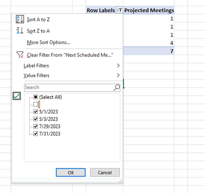
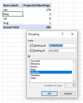
Hi there. I have a formula auto-calculating the next date to a column on which I have a pivot table. I have verified that the dates are valid based on the calendar and that there are no unallowable values that are not formatted as a date. What's also strange is that in the pivot table filter, the box for the blank cells isn't tagged as 'Blank' as it normally is when the cells are blank, but if fact, there is no tag. Further, when I uncheck the box that should be tagged as 'Blank', a little red rectangle appears. I have never seen this before, and cannot understand why I can't group the section. Lastly, I am able to group other pivot tables in that same worksheet from the same source data set, so it's really not an issue of traditional vs. OLAP-based Power Pivot. I added some screen shots below of the data and what I'm seeing. Any insight would be appreciated! Thanks.
- Labels:
-
Excel
- Mark as New
- Bookmark
- Subscribe
- Mute
- Subscribe to RSS Feed
- Permalink
- Report Inappropriate Content
Feb 02 2023 08:04 PM
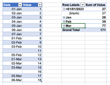
@dharbison For the grouping to work ALL rows must be dates or truly blank. And when you have blanks, the will show up in a group "less than the earliest date in the list". See picture below.
Since you mention that the date column is calculated, I assume you have formula that returns either a date or and empty string (""). An empty string is NOT blank. That's why you see the item with no label and you can not group de dates anymore.
- Mark as New
- Bookmark
- Subscribe
- Mute
- Subscribe to RSS Feed
- Permalink
- Report Inappropriate Content
Feb 03 2023 04:35 AM
Thank you. My formula =IF(H3=3,D3+90,IF(H3=6,D3+180,IF(H3=9,D3+270,IF(H3=12,D3+360,""))))
is returning "" . I guess I've never before tried to group a selection with "" in it.
Thanks for your help!
- Mark as New
- Bookmark
- Subscribe
- Mute
- Subscribe to RSS Feed
- Permalink
- Report Inappropriate Content
Feb 03 2023 04:51 AM - edited Feb 03 2023 04:52 AM
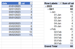
@dharbison Not sure if it's acceptable to you but a workaround could be to return 0 in stead of "". That will create a non-sense date 0 January 1900. Use a custom format to display dates, for instance, as
dd/mm/yyyy;;
The two semi-colons at the end force a 0-date to be displayed as a blank. Then, the pivot table will still group dates by year, quarter and month. Filter out the year 1900 and you can create something like this:
- Mark as New
- Bookmark
- Subscribe
- Mute
- Subscribe to RSS Feed
- Permalink
- Report Inappropriate Content
Feb 03 2023 05:04 AM


