- Home
- Microsoft 365
- Excel
- Cannot conditionally format based off of another row.
Cannot conditionally format based off of another row.
- Subscribe to RSS Feed
- Mark Discussion as New
- Mark Discussion as Read
- Pin this Discussion for Current User
- Bookmark
- Subscribe
- Printer Friendly Page
- Mark as New
- Bookmark
- Subscribe
- Mute
- Subscribe to RSS Feed
- Permalink
- Report Inappropriate Content
Jan 26 2023 08:47 AM
I have a date column in which the date is manually entered. It is currently formatted to turn the text red if equal to or past the due date. This same spreadsheet also has a status column which contains a data validated list of statuses.
I have been given the task to change the date font colour back to black when the status is complete.
I have tried to format it using this formula:
However every formula I try comes back with the same error:
What do I need to do in order to get the date to change back to black font colour?
Any help at all would be greatly appreciated.
- Labels:
-
Excel
-
Formulas and Functions
- Mark as New
- Bookmark
- Subscribe
- Mute
- Subscribe to RSS Feed
- Permalink
- Report Inappropriate Content
Jan 26 2023 09:02 AM
- Mark as New
- Bookmark
- Subscribe
- Mute
- Subscribe to RSS Feed
- Permalink
- Report Inappropriate Content
Jan 27 2023 02:42 AM
@OliverScheurich Ok that has allowed the formula to go in but the date is still formatting as red when the status is "Complete".
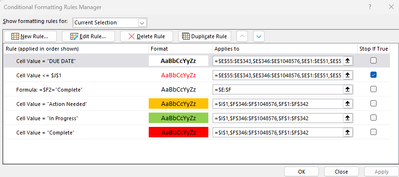
Here is the current arrangement of conditional formats:
I have tried moving the order around and selecting and deselecting 'Stop if True' to see if it will change the font colour but nothing seems to work.
Basically I just need the date font to be red if on or past todays date (which is the part that is working) but I want it to change to black font colour once the status in the STATUS column is "Complete".
Any help that anyone can give is appreciated.
- Mark as New
- Bookmark
- Subscribe
- Mute
- Subscribe to RSS Feed
- Permalink
- Report Inappropriate Content
Jan 27 2023 03:59 AM
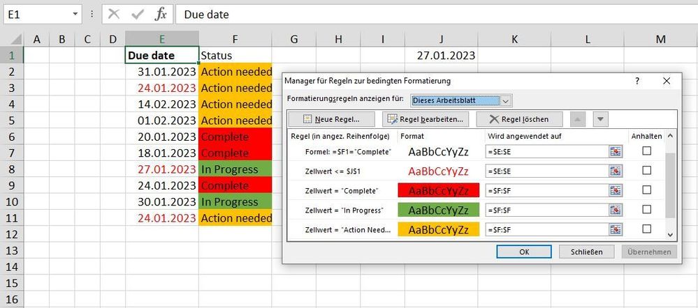
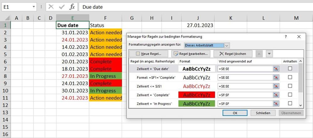
You can try these rules and "applies to" ranges which return the expected result if i correctly understand what is intended. Attached is my sample workbook. The screenshots show all rules and "applies to" ranges. The difference seem to be the "applies to" ranges and =$F1="Complete" instead of =$F2="Complete" and the hierarchy of =$F1="Complete" and <=$J$1.


