Calculate date in a specific product list

[RobinJakobsson123]

Hi,

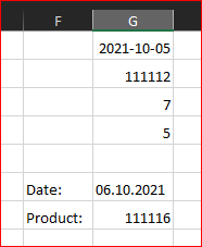
I would need to be able to calculate a shortage date/time. Attached document represents all assembly product starts in a factory. Based on what the user/vlookup will enter in G1-G4, I would like to return the product number in this list and the start position of the day .

As an example, the user enter a shortage: 111112

So with 7+5 positions ahead I would like this script to return:

Date: 6/10

Product: 111116

1:st product start of the day.

I guess that one solution could be a VBA that counts down the column only where format is "XXXXXX".

(And the layout of the excel product list can unfortunately not be changed/redesigned).

[#2]

@RobinJakobsson123 

Please describe in more detail what your plans are.

Welcome to your Excel discussion space!

Thank you for your understanding and patience

Nikolino

I know I don't know anything (Socrates)

[#3]

@NikolinoDE Hi,

G2 = 111112

This is the product I want to start the calculation from. Then calculate 7+5 (G3 + G4 number of steps) down the list and return the new product number, date and number of productstart of that day.

G columns are where the user will enter the data.

[#4 · Accepted solution]

@RobinJakobsson123 

For that layout

it could be

Product:

=INDEX(FILTER(C:C, C:C <> ""),XMATCH($G$2, FILTER(C:C, C:C <> "") )+$G$3+$G$4)

Date:

=INDEX(A:A, XMATCH(0, C1:INDEX(C:C, XMATCH(  G7,C:C))+0,0,-1) )

[#5]

@Sergei Baklan 

Wonderful, that works. Just had to change all the ',' to ';'

The list is in another excel sheet. How do I change the path from C:C to Sheet1!C:C ?

[#6]

@RobinJakobsson123 

Exactly as you said

=INDEX(
   FILTER( Sheet1!C:C, Sheet1!C:C <> ""),
   XMATCH( $G$2,
           FILTER(Sheet1!C:C, Sheet1!C:C <> "")
   ) + $G$3+$G$4
)

and

=INDEX(
  Sheet1!A:A,
  XMATCH( 0,
          Sheet1!C1:INDEX( Sheet1!C:C, XMATCH(  G7, Sheet1!C:C))+0,
          0,
          -1)
 )

Please check in second sheet attached.

The only I'd do not use entire columns in formulas - better named ranges, dynamic ranges or simple range with some gap for future expansion.

[#7]

@Sergei Baklan Thank you very much, very helpful.

How do I calculate the number of start that day? So if the product number is the 3rd start in the list 2021-10-02, I want the function to return only '3'.

And I discovered another issue. I have made dropdown menus in my table. When I expand (adding a row) the dropdown doesn't follow, also the borders I've made. How do I change that?

And this changes when I am expanding the table, in a way that I do not want it to change.

=INDEX(Startprogram!A:A; XMATCH(0; Startprogram!C5:INDEX(Startprogram!C:C; XMATCH( [@[Product no]];Startprogram!C:C))+0;0;-1) )

BR

[#8]

Thank you for your help. Do you have any solution for:

How do I calculate the number of productstart that day? So if the product number is the 3rd start in the list 2021-10-02, I want the function to return only '3'.