Build a dynamic list based on other cell value

[ezequiel2235]

Hi,

I have a list of 5000 records with names of cities (list 1). The user needs to select one but given the size of the list it is difficult to find it. Is it possible to build something that creates a limited list if the user write 3 letters from the city on other cell? For example the list contains these values:

Ārba Minch’, Ethiopia

Arbatache, Boumerdes, Algeria

Arbroath, Scotland, United Kingdom

Arbutus, Maryland, United States

If in the cell A1 the user insert 'ARB' I'd like the list to display only the four values above. is that possible?

Thanks,

Ezequiel

[#2]

@ezequiel2235 

It is possible. Depending on the layout of your workbook/spreadsheet you might want to do this in a very open area, since the number of rows that could be returned could vary a lot.

The FILTER function would work to accomplish what you're asking. If you can without disclosing any confidential information) upload a copy -- or a sample -- of your data, I (or somebody else) can surely create an example.

[#3]

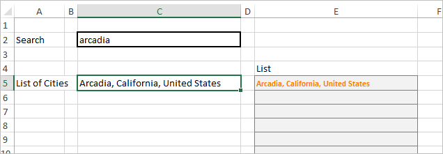
@mathetes Thanks for the reply. I'm attaching a sample of the data. Now the list on C5 is the complete list of cities. I'd need to have the list only displaying those cities that contains the string inserted on the cell C2. I'd appreciatte the support

Ezequiel

[#4]

@ezequiel2235 

Here it is. FILTER worked (although I had to disable the data validation you'd put in that cell for some reason!!)

I've only recently learned how to use FILTER, and it's one really neat function.  I'll be interested in your reaction after you try it with all 500 records. Right now it's set to only work with three character search functions. You could modify it with some sexy additional functions so that you could use variable length search strings, but let's start simple.

[#5]

@mathetes Thanks! super helpful. Only one question to adapt your excel to mine. Should I enter the function as a array? How do I do it? Control+Shift+Enter?

Ezequiel

[#6]

@ezequiel2235 

I know I did NOT enter it with any special flourishes.

Part of the magic of FILTER (that I'm just discovering) is that it takes care of filling the adjacent cells down and to the right, as needed (based on the dimensions of the array you are filtering). I have one of my own where I enter the FILTER function in one cell and it fills the cells down as many rows as needed, and 23 columns to the right. 

You will need to adjust the array that it searches with the full dimensions (or the name of the array) of your 5,000 cities.   If you have country and other data as separate adjacent cells in that 5,000 row table, you might want to retrieve there data too, but just make sure you provide sufficient space for it to "spill" as much as needed.

[#7 · Accepted solution]

@ezequiel2235 

"Legacy" variant

=IFERROR(INDEX(cities[City],AGGREGATE(15,6,1/(LEFT(cities[City],LEN($C$2))=$C$2)*(ROW(cities[City])-ROW(cities[[#Headers],[City]])),ROW()-ROW($E$4))),"")

(regular formula, just drag it down)

I'd modify the Filter as

=FILTER(cities[City],LEFT(cities[City],LEN($C$2))=$C$2,"No match")

[#8]

@Sergei Baklan 

Yes. That addition of LEN was what I had in mind to make it more widely functional, but I was also trying to begin "simple". :)