Automating values inside a column

[Mrinal1996]

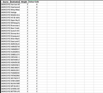
Hi! I have been learning to use the Excel software . I am trying to create a column named "Colour Code" which represents a number based on another column called "Weight". I need to automate this process since the number of columns are large.For eg: if the Weight shows 3, I need to have the numerical "3" in my Color Code list.

How do I go about this? Hoping to hear from you soon.

Excel

Office 365

Formulas and Functions

[#2]

Hello,

Your IF formula will be as such
=IF(C2=3,3,0)

[#3]

@Abiola1 So when I try doing that I am not geting the values on my excel sheet.

 

 

[#4]

Its better to attach the file than pictures

[#5]

@Abiola1  Hi! I am sorry for that. I will attach the file along with this message.

[#6]

Hi @Mrinal1996 

There are several values in the weight column, what do you want the colour code column to return for each value?

If you want the colour code column to only return a specific value only when the weight column value is 3, then you can use the formula earlier suggested by @Abiola1. However, it appears you were trying to achieve a different result based on the values currently on the attached worksheet.

Are you able to provide more information to guide in the appropriate solution?

I have however included the 2 formula in the worksheet to achieve the following:

i. Reproduce the same value under colour code based on information from weight column

ii. Only show 3 when the values in weight is 3, and 0 when different from 3 using

=IF(C2=3,3,0)

Cheers

[#7]

@wumolad Hey thabkyou for working on this.SO basically what I wanted to do was the latter but in a refined form, as in,  all the weights with label "2" should have colour code as 1 , weight "3" as colour code 2, etc.

This i=one is fine as well but if I were to label(colour code) ,say, weight , "128" as "7", how do i do that?

Hoping to hear from you soon.

Regards,

Mrinal Subash

[#8]

It appears there is no uniform pattern based on your criteria, hence, if you want to use one formula for the result, you might need to properly define the output.

The first part looks like weight column value minus 1. Where as you also want 128 to return 7. Are you able to list out all the options you are considering?

You can actually use something like cell D2 should contain

= C2 - 1
Whereby 3 in weight column returns 2 in colour code column.

For the 128, you can use

=IF(C2=128,7,0)
which will return 7 for 128 in weight column and 0 is different from 128.

You can replace 0 with another number incase you dont want it to be 0.

If you are able to list out all the options you are considering, you can use just one formula to address them.

Cheers

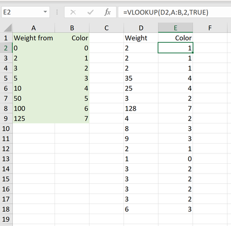
[#9 · Accepted solution]

@Mrinal1996 I believe that you first need to create a table with weight codes and their matching color code. Something like in the attached picture, where the green areas contains the weight/color table. Column D has the weights and column E looks up the corresponding color code from the weight table.

[#10]

@Riny_van_Eekelen Thankyou for this .I think this is the right way to go about it. How do I create that green table ? Just by inserting table on the side? Also may I know what thew parameters denote in the VLOOKUP function that you have in Microsoft Excel?
Regards,
Mrinal Subash

[#11]

@Mrinal1996 The "green table" is no more than two columns with information. One with the weight in the first column and the corresponding color in the second. You can put it anywhere you like. In the same sheet or another.

The VLOOKUP function take has four parameters. 

1. what to look for (the weight)

2. where to look (the "green table")

3. which column to take data from (the second one in the "green table")

4. type of match (TRUE or 1 = approximate match, FALSE or 0 = exact match)

You can read more on VLOOKUP in the MS support pages, here:

https://support.office.com/en-us/article/VLOOKUP-function-0BBC8083-26FE-4963-8AB8-93A18AD188A1