Automate chart data selection

[scheij]

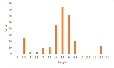
I would like to use a formula to automate Select data..., so that it detects the first and last non-zero value in a series range, then plots one additional category (with series value = 0) before and after them, as shown below and in the attached file.  I considered INDEX/MATCH with OFFSET, but that led to a dead end.  Any suggestions?  Thanks.

[#2]

@scheij  I can't change the automatic function of the select data function but here is a pair of formulas you can paste in a new pair of columns that will 'pull' that range of data for you.  I used a Defined Name "dRange" to define where your data (y-data) is located.  You can either create that NAME in the Name Manager or replace each occurrence with the range you need:

=IFERROR(IF(ROW()=1,"New X",INDEX(OFFSET(dRange,MATCH(TRUE,dRange>0,0)-2,-1,MATCH(TRUE,dRange>0)-MATCH(TRUE,dRange>0,0)+3),COUNT(OFFSET($A$1,0,COLUMN()-1,ROW()-1))+1)),"")

=IFERROR(IF(ROW()=1,"New Y",INDEX(OFFSET(dRange,MATCH(TRUE,dRange>0,0)-2,0,MATCH(TRUE,dRange>0)-MATCH(TRUE,dRange>0,0)+3),COUNT(OFFSET($A$1,0,COLUMN()-1,ROW()-1))+1)),"")

If placed starting in Row 1 it will add the "New X" and "New Y" titles.

NOTE: these are both ARRAY formulas and you must hit CTRL-SHIFT-ENTER after you paste the text in

[#3 · Accepted solution]

@scheij 

You may add two named ranges

Xrange:
=INDEX(Sheet1!$A:$A,AGGREGATE(15,6,1/(Sheet1!$B$2:$B$32<>0)*ROW(Sheet1!$B$2:$B$32),1)-1):INDEX(Sheet1!$A:$A,AGGREGATE(14,6,1/(Sheet1!$B$2:$B$32<>0)*ROW(Sheet1!$B$2:$B$32),1)+1)

Yrange
=INDEX(Sheet1!$B:$B,AGGREGATE(15,6,1/(Sheet1!$B$2:$B$32<>0)*ROW(Sheet1!$B$2:$B$32),1)-1):INDEX(Sheet1!$B:$B,AGGREGATE(14,6,1/(Sheet1!$B$2:$B$32<>0)*ROW(Sheet1!$B$2:$B$32),1)+1)

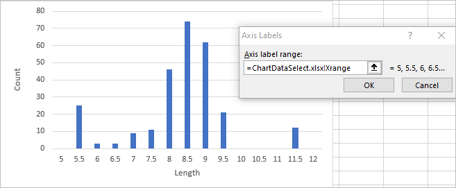
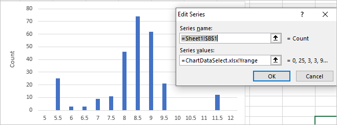
and add use them for chart data

Xrange

Yrange (Series):

[#4]

@mtarler  This remarkable solution achieves much of what I need, but the array formulas seem to "run out of steam" and fail to detect non-zero values in subsequent rows (highlighted in attached workbook).  Changing B20 to a number > 0 extends the array formula results to the next zero value, but not to the last zero as it should.  Thank you for your help.

[#5]

@scheij  apparently I put too much faith in how MATCH() was working.  i tweaked that in the attached.  I also tweaked the dRange name to be more flexible of different lengths of data.

[#6]

@Sergei Baklan 

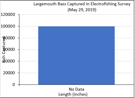
The two named ranges you recommended work great, except in cases with only zero values, when Excel returns this warning.  For example, see X4range and Y4range in Chart 4.

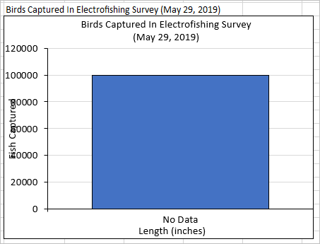
I unsuccessfully tried adding an IF function to create an X category labeled "No Data" and a Y value that's far beyond the expected range.

X4range:
=IF(F5>0,INDEX(Sheet1!$A:$A,AGGREGATE(15,6,1/(Sheet1!$B$2:$B$32<>0)*ROW(Sheet1!$B$2:$B$32),1)-1):INDEX(Sheet1!$A:$A,AGGREGATE(14,6,1/(Sheet1!$B$2:$B$32<>0)*ROW(Sheet1!$B$2:$B$32),1)+1),"NO DATA")

Y4range
=IF(F4>0,INDEX(Sheet1!$B:$B,AGGREGATE(15,6,1/(Sheet1!$B$2:$B$32<>0)*ROW(Sheet1!$B$2:$B$32),1)-1):INDEX(Sheet1!$B:$B,AGGREGATE(14,6,1/(Sheet1!$B$2:$B$32<>0)*ROW(Sheet1!$B$2:$B$32),1)+1),99988)

Any suggestions to accommodate non-zero values and avoid the warnings would be appreciated.  The workbook is attached.  Thanks.

[#7]

@scheij 

We may wrap formulas with IFERROR as

=IFERROR(INDEX(LF!$K:$K,AGGREGATE(15,6,1/(Freq4<>0)*ROW(Freq4),1)-1):INDEX(LF!$K:$K,AGGREGATE(14,6,1/(Freq4<>0)*ROW(Freq4),1)+1),"No Data")

and

=IFERROR(INDEX(LF!$F:$F,AGGREGATE(15,6,1/(Freq4<>0)*ROW(Freq4),1)-1):INDEX(LF!$F:$F,AGGREGATE(14,6,1/(Freq4<>0)*ROW(Freq4),1)+1),99988)

Result is

[#8]

Yes, that's a better fix. Thank you.

[#9]

@scheij , you are welcome

[#10]

@Sergei Baklan 

I made the recommended changes, but the caution message (pasted above) still appears when the formula finds only zero values, as in Chart 4, Xrange4, and Yrange4.   Also, the category axis label does not show "No Data" as expected in the IFERROR function in named formula, Xrange4.  I noticed S133:S134 are entered as array formulas, but I was not able to do that in the Name Manager with shift-ctrl-enter.  Copying any other value from row 4 to F4 produces the expected results with no warning.  Any suggestions would again be appreciated.

[#11]

@scheij 

1) I don't see such error on my version of Excel, however formulas for X4 and Y4 return extra zero, my mistake. Corrected,  -1 and +1 after the AGGREGATE changed on -0 and +0. Or they are could be removed at all.

2) S133 and S134 shall return arrays, these formulas are for dynamic ranges. I assumed you are on Excel with dynamic arrays since in comments XLOOKUP and UNIQUE are mentioned. If open in Excel without dynamic arrays these formulas will be shown as array ones. That's okay, but don't Ctrl+Shift+Enter them in named formulas, that doesn't work. In Name Manager keep them as regular formulas.

Please check attached file. Right now I have no access to pre-DA Excel and can't test on it, hope will work. On DA Excel it works.

[#12]

@Sergei Baklan 

I do not yet have Excel-DA because UNIQUE and XLOOKUP are not available functions.  I read about those new features and noted that they would soon be released, beginning in July 2020.  Hope it arrives soon!

When I tried to download and open your latest version, these messages initially appeared, but I used File, Open from my Downloads folder to open the workbook.  

The warning messages still show when Xrange4 and Yrange4 return only zeros.

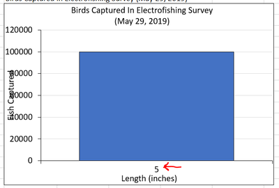
Chart4 appears as... ,but the X category label should be "No Data."

We want to keep the extra zeros before the first and after the last categories, so I changed Xrange4 and Yrange4 to original formulas.

[#13]

@scheij 

To my knowledge deployment of dynamic arrays for Office 365 subscribers is finished, they shall be available for all channels and all platforms.

I opened the file you attached, no errors and chart is correct

What do you see in R132:T133? In my case that is

[#14]

I see the same in R132:T133, and the formulas are arrays enclosed with { }. The cautions still appear, and Chart4 now has no X category label. The 5 value from the last image is gone. I'll check with our company about Office 365 updates that they might have scheduled for us. I sincerely appreciate your help. Thank you.

[#15]

@scheij 

I see, thank you. Will try to play with that bit more, will update you if find something.

[#16]

Our agency plans to distribute the new release later this month after testing and approval. I'll let you know if the caution continues with Excel-DA. Thanks again for your help.