Auto-populate a cell with the contains from another cell

[stephurso]

Hello:

I have a spreadsheet that I would like to auto-populate information to a cell from another cell. 

Example.  In B2 I type in 4122 and select Enter.  The text description for item 4122 (its a long part description) is in C62 (on the same spreadsheet).  When I type in the 4122 into B2 I want it to display the text from C62.  I will need this for 55 items so if someone types in 4233 into B2 then it will reference that cell for that part description.  Not sure if this is a IF Then or statement. 

Currently users have to manually cut and paste or add the part description in and I want to automatic that as much as I can to avoid human data errors. 

Thank you in advance.

Steph

[#2]

@stephurso Create a lookup table as demonstrated in the attached file. Depending on your Excel version you might be able to use XLOOKUP. Otherwise you'll have VLOOKUP or INDEX/MATCH at your disposal.

[#3]

Hello: @Riny_van_Eekelen 

This worked great! I used the VLOOKUP formula.  Just one question.  When there is no part number in B2, C2 displays #N/A.  Is there a way to suppress that so it's just blank until someone actually puts in a part number into B2?

[#4]

@stephurso Then you can wrap the lot in an IFERROR, like this:

=IFERROR( vlookup-formula , "" )

[#5]

Like this? =IFERROR(VLOOKUP(B2,Parts,2,FALSE)

I keep getting an error message.

[#6 · Accepted solution]

@stephurso In te file I sent you the formula would become:

=IFERROR(VLOOKUP(B2,Parts,2,FALSE),"")

See attached.

[#7]

Worked like a charm. One more item while I have you. Is there a way to force the format of the part description to the cell? in the order section some words are bold and or highlighted in red. When I type in a part number such as 4122 the description shows but the formatting does not. Everything is just lowercase with no bold or words with color. Not a big deal but it would be nice.

[#8]

@stephurso Unfortunately, not something I can help you with. If possible you probably need VBA to do so.

[#9]

No worries understood. Regarding this code that you supplied which works wonderful. It is possible to add a function that if the user does not add a valid part number (one that is not in cells B11 through B65 then it would display "Not a valid Part Number"?

=IFERROR(VLOOKUP(B2,Parts,2,FALSE),"")

[#10]

Try this:
=IFERROR(VLOOKUP(B2,Parts,2,FALSE),"Not a valid Part Number")
Best of luck

David

[#11]

@Riny_van_Eekelen 

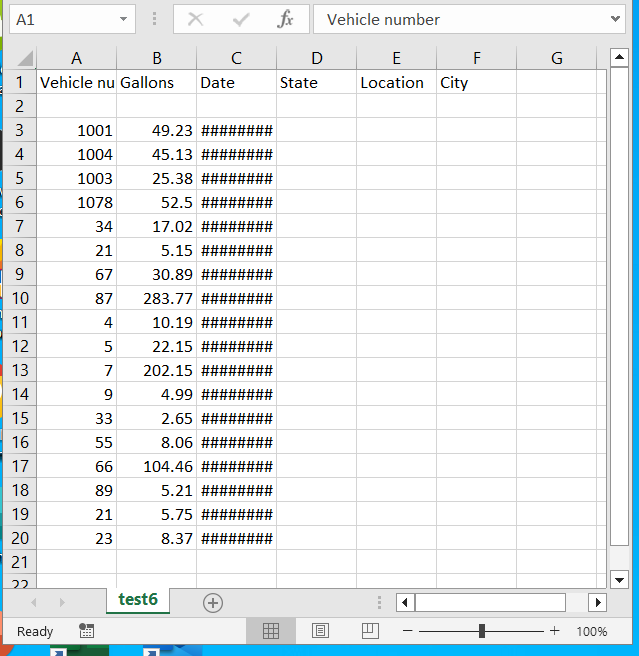
Hello. I have a spreadsheet that records fueling info for a truck company. It contains 3 columns of data, such as Vehicle #, Gallons, Date.  note: I am actually currently using an excel to re-arange the data in this required order shown in attached photo.     

The file is downloaded from the fuel recorder once per day. It contains different quantity of rows each day. Example today may have been 20 rows of data, tomorrow 35 rows.  There is no static data in any cell. 

I now need to add 3 additional columns of State (KY), Location (LOT) and City (Nashville).  This will be static data. My issue is that this data only needs to populate down to where the entries end. As I said, they end in different rows each day. Example: If the file only contains data down to row 20, then my 3 new static fields should not populate past 20.

I need a formular or excel script to look at the cell to the left and if its populated with any data, then add the 3 static fields. If not populated, leave blank. 

Thanks

Randy

[#12]

@OwenRandy214 Your question isn't related to this old thread. Best to open a new discussion.