Auto fill color in based on its value

[davidmillercrawfordusa]

Simple ask (I hope): I want to color an "average of total" cell at the bottom of a column populated with a number of 1 to 4. A different color for less than 2, between 2&3, between 3&4, and between 4&5.

ANy help appreciated!

[#2]

@davidmillercrawfordusa 

=AND(A12>=2,A12<=3)

You can try this rule for conditional formatting (yellow in the example).

=$A$12:$D$12

This is the range the formatting applies to in the example.

[#3]

@davidmillercrawfordusa 

thank you I will give this a try!

[#4]

I'm a novice (and I can't read German), could help with a step-by-step instruction?

[#5]

@davidmillercrawfordusa 

I've attached a sample file which should show everything in english on your computer.

Let's say you want to apply conditional formatting to cells A12:D12.

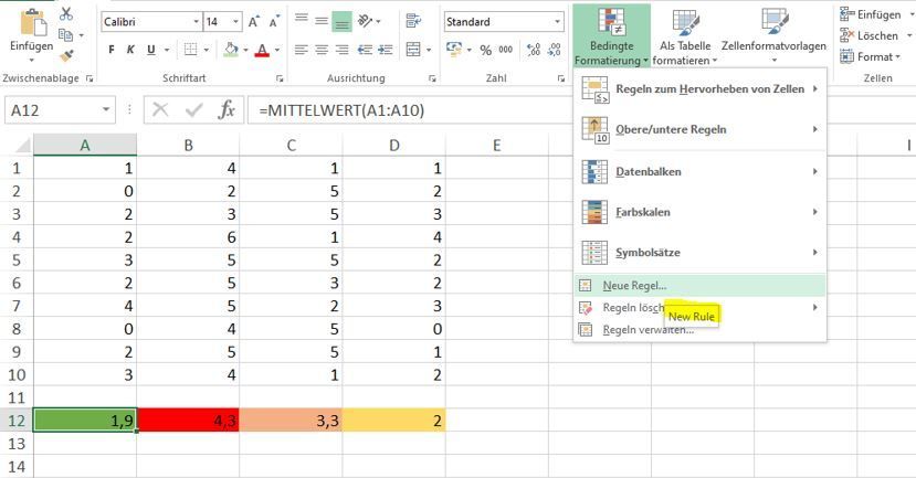
Then select the range A12:D12 with the mouse and then select "conditional format" (Bedingte Formatierung) -> "new rule" as shown in the screenshot.

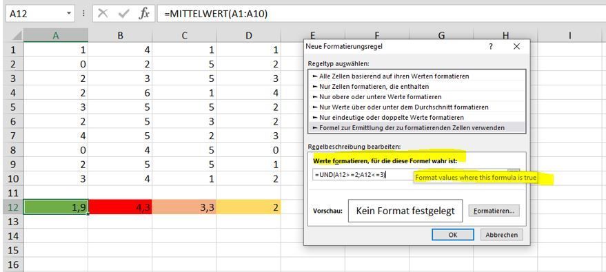
Then "use a formula to determine which cells to format"

Then "format values where this formula is true"

After entering the rule for conditional formatting ( =UND(A12>=2;A12<=3) in the screenshot below, translated:  =AND(A12>=2,A12<=3)  ) you can click on format.

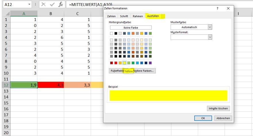
Then you can select the format and then click "Ok" two times.

[#6]

Thank you and danke schön!