Auto Adjust cell color, if previous cell is bigger or smaller number.

[Antoniou_Thanasis]

Hello, 

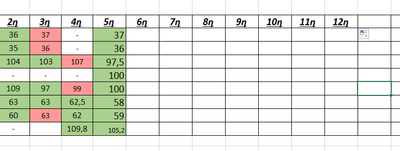
I want to add colours on the table below automaticaly. I know how to do it using conditional formating. I would like to know if it is possible for the cell to get a color automatically when I enter new numbers in the table. I would like the function to calculate the previous cell and not with a predefined value. For example, if in the 6th column, first row, I enter the number 36, the color will turn green, while if I enter 38, it will turn red, because the previous value is 37.

[#2]

@Antoniou_Thanasis 

What are the - in some of the cells?

Do those cells contain 0, formatted to display - ?

Or is it just the text value - ?

[#3]

it is just text value -. i can leave it empty if it helps. I just dont value for those cells.

[#4 · Accepted solution]

@Thanasis_Antoniou 

Select the cells that you want to format. In the following, I will assume that C3 is the top left cell of the selection, and that it is the active cell in the selection.

On the Home tab of the ribbon, click Conditional Formatting > New Rule...
Select 'Use a formula to determine which cells to format'.
Enter the formula

=NOT(AND(ISNUMBER(B3),C3>B3))

Remember, C3 is the active cell, and B3 is the cell to the left of that.

Click Format...
Activate the Fill tab.
Select Green.

Repeat these steps, but with the formula

=AND(ISNUMBER(B3),C3>B3)

and Red.
Click OK, then click OK again.

[#5]

@Hans Vogelaar 

It Works! i also created 2 rules for empty or "-" cells to be default color. Check the image.

Thanks you very much