Array partial matching with VLOOKUP

[Nosmeister]

Good day everyone,

I'm attempting to use a function similar to VLOOKUP, but instead of searching for a single criteria, I'm looking to get a partial match from one array to another. I've illustrated my end goal hopefully a little bit clearer within my attachments.

Without disclosing specifics, I'm essentially tracking automated moves for personnel accounts to and from physical destinations across the country. I would like to have a Conditional Formatting rule to highlight moves that should be in progress but are stuck in the report so that I can manually investigate and escalate for intervention if needed. I have two tables populated from outside sources via power queries: 

One for the tickets and moves themselves and one for the current status of certain key units that they're moving to and from.

The thing that makes this extra complicated to me is that the matches have to be partial. That is to say site information is something like "ALPHA" and I have to find that within a list of information that might say "ALPHA STREET." I've also illustrated this in my example.

The real spreadsheet I'm using is Macro-enabled with PII and a lot more going on behind the scenes, so I created a mockup for this one particular issue I'd like some help with. I've been beating my head on a wall with this for months, eventually conceding to manually going through and highlighting them by hand. I don't know what function I need or if it's even possible.

With my work environment, it's not possible for me to install addons or additional scripts but like I said, macros and power queries are okay. Thank you for any insight into this hopefully simple issue. If it can't be solved with a simple Conditional Formatting formula, then maybe I'll have to dive into VBA.

[#2]

@Nosmeister 

Forgive me for my inability to wrap my head around all the conditions you're testing for here. I do this purely as a volunteer, and sometimes will spend quite a bit of time trying to get through a quandary such as yours.

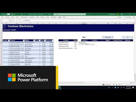
What I've read, though--convinces me that you may just need to be pointed in a different direction, since you clearly have a fair amount of Excel ability already. Are you aware of the new Dynamic Array functions? Notably FILTER?

FILTER, like VLOOKUP, can search through a table and find matches....unlike VLOOKUP--this is where it gets exciting--FILTER can combine multiple criteria and find multiple matches, yielding a list of the rows that meet said multiple criteria.

It seems to me that using FILTER, with criteria working to yield a separate list of the rows that match, you can just produce that list on a sheet of its own, dynamically (as conditions change) and forget Conditional Formatting. Take a look at this video (you will need the most recent version of Excel for these Dynamic Array functions to work): https://www.youtube.com/watch?v=9I9DtFOVPIg

[#3]

@Nosmeister 

Conditional formatting rule formula for GO could be

=SUM( COUNTIFS($C2:$D2,"*"& INDIRECT("Table2[NAME]") &"*") * ( INDIRECT("Table2[STATUS]") = "GO") ) * ( $E2 <= TODAY() )

 Similar for NO GO

Not sure I understood the logic correctly. You speak about OR logic. With that not clear which rule to apply. Name with GO could be New Unit and at the same time Name with NO GO - in the Old Unit in same row.

[#4]

@mathetes 

Thanks so much for the reply. I've been learning the beast that is excel at my own pace out of necessity and until now I'd never heard of the FILTER function. It'll take some tinkering on my end to get to know it but that's all I was asking for; a nudge in the right direction.

[#5]

@Sergei Baklan 

That's certainly better than anything I'd come up with in the past 3 days of working with this, thank you so much. The closest I'd managed to get was something like this:

=VLOOKUP($C2,SiteStatus!A2:B14,2,TRUE)="GO"

...but that only ended in confusion. I think it was the partial match condition that was giving me the hardest time. It was the closest I could get though.