Apply Pivot Table on selected items with addition filter of billed in current quarter only

[vt_excel]

1. Below is image of data set on which I have to apply pivot. For reference I gave 3 sets, actually it can go upto 5000

2. Conditions are:
a) Customer name, manufacturer & item name should be same
b) total billing should >= 3000
c) One of Billing should happen in this current quarter, like in current scenario from 1-July-22 to 31-sep-22. So it could be case that part billed is >=3000 last year, but if in current quarter even if 1 dollar is billed, then it should count

3. Attached image, Robert should appear in end result since its billed in this quarter & total value is >=3000

4. How to do that? I can apply Pivot on rest of columns, but this condition that there should be some billing in this quarter, how to do that?

Customer Name	Manufacturer	Item	Bill date	Amount
Robert	Newway	Apple	15-Jul-22	1500
Jass	Highend	Orange	10-Dec-21	4000
Robert	Newway	Apple	07-Jan-20	1500
End Result
Customer Name	Manufacturer	Item	Bill date	Amount
Robert	Newway	Apple	15-Jul-22	1500
Robert	Newway	Apple	07-Jan-20	1500

[#2]

Could you please attach the dataset with a few more records.. kindly attach the excel file
Regards, Faraz

[#3]

@vt_excel Not sure that a pivot table is what you need. I created something in Power Query that seems to achieve the desired output, based on the conditions you mentioned. See if you can get it to work on your real data.

[#4]

Hi Riny_van_Eekelen
How you have used power query and what filer/formula applied? I will check at my excel too.

[#5]

@vt_excel Well, when you open the Advanced Editor in Power Query, you can see the applied steps that take you from the blue table to the green one. It's not very straight-forward if you haven't worked with PQ before. Have you?

[#6]

@Riny_van_Eekelen Thanks for reply.

Havent worked in PQ before. 

Can you suggest some right links, i am searching online also..

[#7]

@vt_excel The site in the link below, would be a good place to start.

https://exceloffthegrid.com/power-query-introduction/ 

[#8]

@vt_excel 

This is intended to achieve the same result using a 365 formula

= LET(
      inQtr, COUNTIFS(
         Table1[Customer Name], Table1[Customer Name],
         Table1[Manufacturer],  Table1[Manufacturer],
         Table1[Item],          Table1[Item],
         Table1[Bill date],     ">=" & DATE(2022,7,1),
         Table1[Bill date],     "<=" & DATE(2022,9,31)
      ),
      total, SUMIFS(Table1[Amount],
         Table1[Customer Name], Table1[Customer Name],
         Table1[Manufacturer],  Table1[Manufacturer],
         Table1[Item],          Table1[Item]
      ),
     FILTER(Table1, (inQtr>0)*(total>=3000))
   )

Without LET and FILTER you would need helper columns (or Power Query of course)

[#9]

@vt_excel 

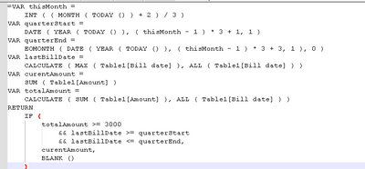
If with PivotTable - creating it we may add data to data model and use measures

Filtered Amount :=
VAR thisMonth =
    INT ( ( MONTH ( TODAY () ) + 2 ) / 3 )
VAR quarterStart =
    DATE ( YEAR ( TODAY () ), ( thisMonth - 1 ) * 3 + 1, 1 )
VAR quarterEnd =
    EOMONTH ( DATE ( YEAR ( TODAY () ), ( thisMonth - 1 ) * 3 + 3, 1 ), 0 )
VAR lastBillDate =
    CALCULATE ( MAX ( Table1[Bill date] ), ALL ( Table1[Bill date] ) )
VAR curentAmount =
    SUM ( Table1[Amount] )
VAR totalAmount =
    CALCULATE ( SUM ( Table1[Amount] ), ALL ( Table1[Bill date] ) )
RETURN
    IF (
        totalAmount >= 3000
            && lastBillDate >= quarterStart
            && lastBillDate <= quarterEnd,
        curentAmount,
        BLANK ()
    )

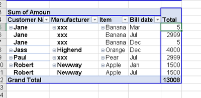
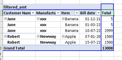
Result is

[#10]

@Peter Bartholomew 

So, we have full set of solutions except one for legacy Excel. Most probably it could be done with AGGREGATE(), but I'm lazy to generate it now.

[#11]

@Sergei Baklan 

Thanks for ur detailed response.

1. I tried applying pivot table, but where & how to add filtered_amount column in it.

below is screenshot of pivot table i applied

2. Also if i direclty add bill_date in pivot table, it get broken into month, qtr & year.

what i do is first  i change date format to number, apply pivot & then change format again to date. that way i can see full date dd-mm-yy in pivot.

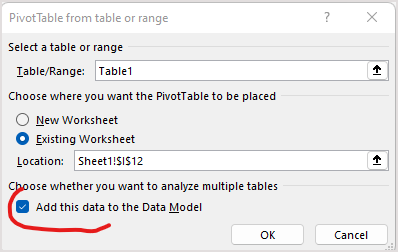
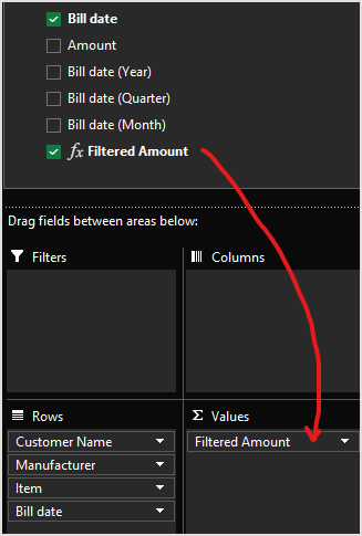
[#12 · Accepted solution]

@vt_excel 

Let assume you your Excel version/platform supports data model. Creating PivotTable you need to add data to data model:

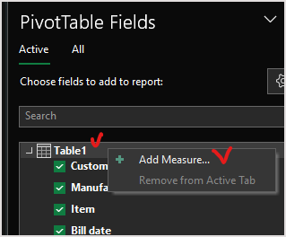
Right click on table name In PivotTable Fields pane and Add measure

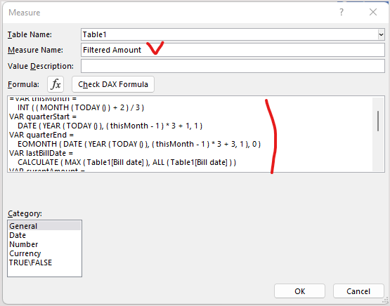
Create DAX measure in opened window

Use this measure in PivotTable for aggregation

[#13]

@Sergei Baklan thanks for your detailed post, been able to get the results

Now understanding this formula line by line

a) first line would get 3

b) second would be qtr start date

c) third would be qtr end date

how does pivot table only takes values which have this qtr date?

[#14]

@vt_excel 

If we have no other filters measure calculates result for the combination of name, manufacture, item, and bill date in the PivotTable row.

Variables quarterStart and quarterEnd depend only on current date.

Variable lastBillDate returns it independently of the date, we removed date filter by ALL ( Table1[Bill date] )

Variable currentAmount sums amount for the combination of field values in PivotTable rows. Actually it's the same if you drag Amount into Values of PivotTable.

Variable totalAmount do the same but ignores Bill date, i.e. total for all dates for the given combination of name, manufacture and item.

Finally we check if totalAmount is more than 3000 and Bill date is within current quarter. If yes, we return currentAmount for the Bill date, otherwise blank value. Rows with blanks are ignored in PivotTable.

As a comment, if we work with defined date, not TODAY(), bit more filtering will be required. No need in it if result is always for the current date.

[#15]

thanks for detailed explanation.

[#16]

@vt_excel , you are welcome