- Subscribe to RSS Feed
- Mark Discussion as New
- Mark Discussion as Read
- Pin this Discussion for Current User
- Bookmark
- Subscribe
- Printer Friendly Page
- Mark as New
- Bookmark
- Subscribe
- Mute
- Subscribe to RSS Feed
- Permalink
- Report Inappropriate Content
Oct 05 2021 09:25 AM
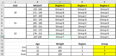
Help needing to create a formula that would automatically filter data on E13 to E15 based 3 or more criteria as shown below and attached (excel is a mockup to keep actual work data private).
challenge I am having is that info on column B has a range that I can't use a Vlookup with it.
- Labels:
-
Excel
- Mark as New
- Bookmark
- Subscribe
- Mute
- Subscribe to RSS Feed
- Permalink
- Report Inappropriate Content
Oct 05 2021 11:13 AM
See the attached version. I unmerged the cells in column A and repeated the ages, and I split the weight ranges into two columns.
- Mark as New
- Bookmark
- Subscribe
- Mute
- Subscribe to RSS Feed
- Permalink
- Report Inappropriate Content
Oct 05 2021 03:42 PM
- Mark as New
- Bookmark
- Subscribe
- Mute
- Subscribe to RSS Feed
- Permalink
- Report Inappropriate Content
Oct 05 2021 07:16 PM
Solution
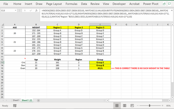
The formula is:
=INDEX(($B$2:$E$4,$B$5:$E$7,$B$8:$E$10), MATCH(C13,VALUE(SUBSTITUTE(INDEX(($B$2:$B$4,$B$5:$B$7,$B$8:$B$10),,,MATCH(B13,FILTER(A2:A10,(A2:A10>1)*1),0)),RIGHT(INDEX(($B$2:$B$4,$B$5:$B$7,$B$8:$B$10),,,MATCH(B13,FILTER(A2:A10,(A2:A10>1)*1),0)),6),)),1),MATCH("Region "&D13,$B$1:$E$1,0),MATCH(B13,FILTER(A2:A10,(A2:A10>1)*1),0))
cheers
- Mark as New
- Bookmark
- Subscribe
- Mute
- Subscribe to RSS Feed
- Permalink
- Report Inappropriate Content
- Mark as New
- Bookmark
- Subscribe
- Mute
- Subscribe to RSS Feed
- Permalink
- Report Inappropriate Content
Oct 06 2021 11:28 AM
Accepted Solutions
- Mark as New
- Bookmark
- Subscribe
- Mute
- Subscribe to RSS Feed
- Permalink
- Report Inappropriate Content
Oct 05 2021 07:16 PM
Solution
The formula is:
=INDEX(($B$2:$E$4,$B$5:$E$7,$B$8:$E$10), MATCH(C13,VALUE(SUBSTITUTE(INDEX(($B$2:$B$4,$B$5:$B$7,$B$8:$B$10),,,MATCH(B13,FILTER(A2:A10,(A2:A10>1)*1),0)),RIGHT(INDEX(($B$2:$B$4,$B$5:$B$7,$B$8:$B$10),,,MATCH(B13,FILTER(A2:A10,(A2:A10>1)*1),0)),6),)),1),MATCH("Region "&D13,$B$1:$E$1,0),MATCH(B13,FILTER(A2:A10,(A2:A10>1)*1),0))
cheers


