2 way lookup

[mark76]

Hi,

I am trying to look for products from column B in column F. Once found I want to compare the 'capacity' with 'quantity'. If quantity is less than capacity for that product I want to display location, product code and quantity for that item.

Can this be done with INDEX and MATCH or will I have to use something else?

[#2]

@mark76 

In column B there are few entries for each product code. If found, sum quantity for all locations to compare with capacity?

 "..to display location, product code and quantity"  - product code is already displayed in column F. Where to display location and quantity?

Better to attach the sample with manually generated result, it'll be much easier to understand what is required.

[#3]

@Sergei Baklan

 In column B there are few entries for each product code. If found, sum quantity for all locations to compare with capacity?

No, I need to compare each one and display the results.

 "..to display location, product code and quantity"  - product code is already displayed in column F. Where to display location and quantity?

Although product code is displayed in column F that column is fixed and i need to re-display product code from column B along with location and quantity in another table.

I have attached my worksheet.

[#4 · Accepted solution]

@mark76 

Thank you for the update. With that perhaps like

=IFERROR(INDEX($B$2:$B$8,AGGREGATE(15,6,1/($C$2:$C$8<=INDEX($G$2:$G$12,MATCH($B$2:$B$8,$F$2:$F$12,0)))*(ROW($B$2:$B$8)-ROW($B$1)),ROW()-ROW($K$1))),"")

Please check in attached.

[#5]

@mark76 

As an alternative:

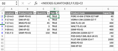
If you can accept a solution that simply filters the items that match your criteria, you could do the following. Introduce a helper column D to check the criteria en enter

=INDEX(G:G,MATCH(B2,F:F,0))>C2

in D2. Copy the formula down to the bottom of your list and filter it on TRUE.

In your example, filtering on the first table will also hide row 5 from the second table because you have  them side-by-side. Probably an unwanted situation. So if it works for you not having both tables in the same sheet and side-by-side (thus move the second table somewhere else), this is an easy solution. Obviously, you need to update the column references for G and F to their new location.

[#6]

@Sergei Baklan 

@Riny_van_Eekelen 

Thank you both :)