Need help: How to Transform data from combined lists to separate options

[Sally Lim]

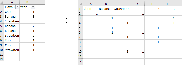
Hi, does anyone know if there's an efficient way to transform columns of data as seen in left image below to a new set that looks like image on the right? 

[#2]

This looks like it could be solved with an IF statement:

=IF($A2="","",IF($A2=C$1,1,"")) for flavours.

=IF($A2="","",IF($B2=F$1,1,"")) for years.

[#3]

Hi Sally,

please find attached my attempt to solve it using Power Query. The query automatically extracts the names of flavours and creates up to 3 flavour columns and 3 years. If you wish to add extra flavours, you would need to add them into the query. Alternatively, you could setup a custom function, which would automatically add flavour columns (and years) based on the number of flavours.

Here is the query, assuming that your initial table is named tblSource

let
   
    //Create list of flavours 
    Source = Excel.CurrentWorkbook(){[Name="tblSource"]}[Content],
    #"Filtered Rows" = Table.SelectRows(Source, each ([Flavour] <> null)),
    #"Removed Other Columns" = Table.SelectColumns(#"Filtered Rows",{"Flavour"}),
    #"Removed Duplicates" = Table.Distinct(#"Removed Other Columns"),
    Flavours = #"Removed Duplicates"[Flavour],
   
    //Variables to hold flavour names
    Flavour1 = try Text.From(Flavours{0}) otherwise "",
    Flavour2 = try Text.From(Flavours{1}) otherwise "",
    Flavour3 = try Text.From(Flavours{2}) otherwise "",

    //Add flavour and year columns
    #"Changed Type" = Table.TransformColumnTypes(#"Filtered Rows",{{"Flavour", type text}, {"Year", Int64.Type}}),
    #"Added Flavour1" = if Text.Length(Flavour1)>0 then Table.AddColumn(#"Changed Type", Flavour1, each if [Flavour]=Flavour1 then 1 else "") else "",
    #"Added Flavour2" = if Text.Length(Flavour2)>0 then Table.AddColumn(#"Added Flavour1", Flavour2, each if [Flavour]=Flavour2 then 1 else "") else #"Added Flavour1",
    #"Added Flavour3" = if Text.Length(Flavour3)>0 then Table.AddColumn(#"Added Flavour2", Flavour3, each if [Flavour]=Flavour3 then 1 else "") else #"Added Flavour2",
    #"Added Year1" = Table.AddColumn(#"Added Flavour3", "Year 1", each if [Year]=1 then 1 else ""),
    #"Added Year2" = Table.AddColumn(#"Added Year1", "Year 2", each if [Year]=2 then 1 else ""),
    #"Added Year3" = Table.AddColumn(#"Added Year2", "Year 3", each if [Year]=3 then 1 else ""),
    #"Removed Columns" = Table.RemoveColumns(#"Added Year3",{"Flavour", "Year"})
in
    #"Removed Columns"

Hope this helps

Yury

[#4]

Thanks so much Yury! :) Do you know what steps are involved with creating it into a custom function as you mentioned above?

[#5]

Hi Sally,

you need to use a recursive funciton. Please see the attached file for my attempted solution

Here is the text of the function I used:

let
  
    /* This function loops the list of headers and adds new columns to the source table, which match the list */

    fnAddColumnsFromList = (nmb_index as number,
   lst_flavours as list,             /*List of column headers*/
    tbl_source as table ) =>          /*initial source table to append columns to*/

    if nmb_index >= List.Count(lst_flavours) /*iterate only the number of times matching the number of items in the list of column headers*/
   
        then 
            tbl_source     /*end result of the function once the maximum number of iteration is achieved*/
      
        else
            //add new column
            @fnAddColumnsFromList(nmb_index+1,            /*increment index for next iteration*/
                                 lst_flavours,
                                 if Text.Length(try Text.From(lst_flavours{nmb_index}) otherwise "")>0 then Table.AddColumn(tbl_source, Text.From(lst_flavours{nmb_index}), each if [Flavour]=Text.From(lst_flavours{nmb_index}) then 1 else "") else ""
                                 )                                        
                 
in

    fnAddColumnsFromList

Yury

[#6]

That's a very smart solution @Yury Tokarev!

My take would have been to pivot twice like this (that can be done completely through the UI):

let
    Source = Excel.CurrentWorkbook(){[Name="Table1"]}[Content],
    RowNumber = Table.AddIndexColumn(Source, "RowNumber", 1, 1),
    ForFirstPivot = Table.AddColumn(RowNumber, "FirstPivot", each 1),
    ForSecondPivot = Table.AddColumn(ForFirstPivot, "SecondPivot", each 1),
    PivotFlavour = Table.Pivot(ForSecondPivot, List.Distinct(ForSecondPivot[Flavour]), "Flavour", "FirstPivot"),
    PivotYear = Table.Pivot(Table.TransformColumnTypes(PivotFlavour, {{"Year", type text}}, "en-US"), List.Distinct(Table.TransformColumnTypes(PivotFlavour, {{"Year", type text}}, "en-US")[Year]), "Year", "SecondPivot")
in
    PivotYear

[#7]

Thanks Yury! That query is very helpful and I can manage to replicate it with other data manually. However I was wondering if there's a way to apply this query to a new set of data without having to write up the query again manually? And what would you suggest for multiple columns of data rather than just 2?

Appreciate your help!

Sally 

[#8]

Hi Imke,

that is a great solution.

Thank you

Yury 

[#9]

Hi Sally,

could you please give examples of a new set of data you would like to apply the query to, and of the multiple columns of data you woule like to have?

Thank you

Yury