Spreadsheet Help with Formulas Across Several Columns

[John Breeden]

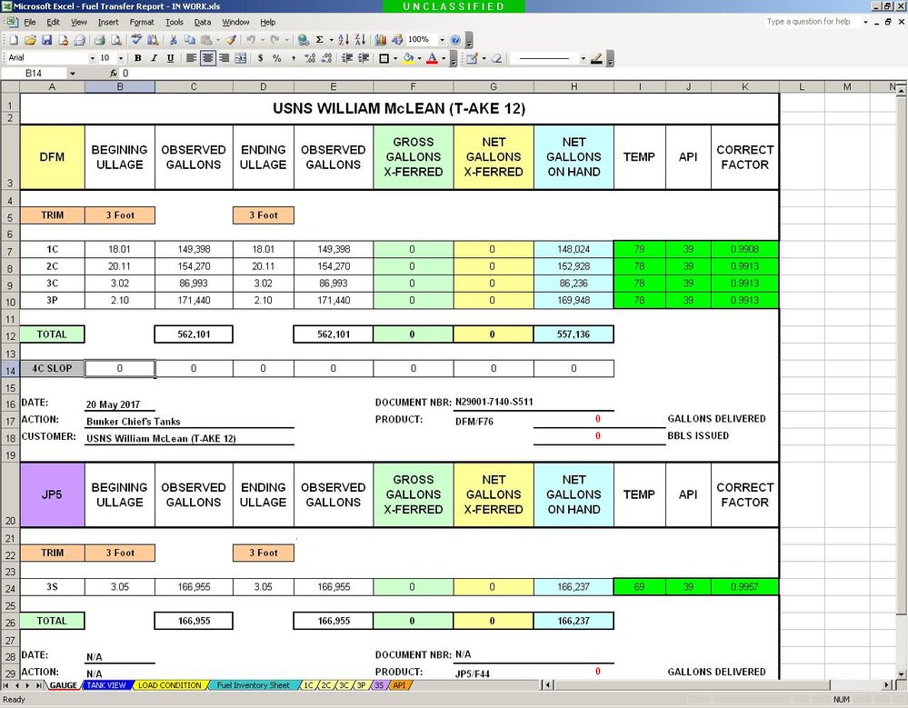
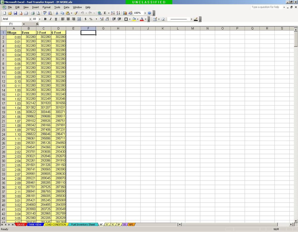
In cell B5 it currently says 3 Foot.  In different scenarios it can also say 6 Foot or Even.  I need cell C7 to reference the appropriate column on tab 1C in regards to Even, 3 Foot, or 6 Foot, then I need it to reference the corresponding number in cell B7 that corresponds to the same number on tab 1C under the Ullage column.

I'm using LOOKUP right now which works fine with only two columns but I need it to work with several columns under different scenarios.  When looking at

Below is tab 1C and the tabs I was talking about which should make this much easier to understand.  Basically, when I enter the Ullage in cell B7 it needs to reference the Even, 3 Foot, or 6 Foot column and give me that number.  For example, the Ullage is 1.03 and the Trim is 3 Foot, the correct number is 302142.  If I can get some help with this I can make the rest of this spreadsheet work because the formula I'm looking for will work for the rest of this spreadsheet.

Also, is there a way to make the Even, 3 Foot, and 6 Foot a dropdown selection instead of having to type it directly in all the time?

My knowlegdge of Excel is severely limited and any help you can provide will be greatly appreciated.

[#2]

Hi John

It's better to provide a workbook than a bunch of photos.

[#3]

I agree completely.  Please see attached workbook.  If you have any questions, please don't hesitate to ask.

[#4 · Accepted solution]

One possible solution:

=INDEX('1C'!A:D,LOOKUP(B7,'1C'!A2:A509,ROW('1C'!C2:C509)),MATCH(B5,'1C'!1:1,0))

[#5]

That worked PERFECT!!!!!!!!!!!!!!!!!!!!!!!!!!!!!!!!!

I have one more problem to solve with the same notebook.

On the main spreadsheet (Gauge), the Columns TEMP, API, and CORRECT FACTOR.  I need cell K7 to get it's information based off the reference points of cell I7 and J7 from tab API.

On the API tab the Temp is the far left column and ranges from 30-119 degrees.

The API column header starts at B1:U1 with the corresponding APIs B2:B91 through U2:U91.

Simply put, I need the Correcton Factor to cross reference the temperature in relation to the API.  This should work similar to the previous problem you just solved for me.

If you have any questions, PLEASE don't hesitate to ask!  YOU'RE A GREAT HELP!!!!!!!!!!!!!

[#6]

This time a slightly different solution.

=INDEX(API!$A$1:$U$91,MATCH(I7,API!$A:$A,0),MATCH(J7,API!$1:$1,0))

[#7]

PERFECT AGAIN!!!!

Sorry for not replying sooner but I was out on a run at the end of the day.  I just checked a few minutes ago this morning and it's perfect!!!!

I've been struggling with this for quite some time now but you cinched it up quickly.

After looking at it I was wondering if there was a way to have the 3 Foot, 6 Foot, and Even in a dropdown box where you currently have to manually type it.  If you could help me with that one it would be a homerun!!!  If not then it's still a homerun because you just don't know how long I've been trying to make this work.

Again, thank you very, very, very much!!!!

P.S.  Whatever your employer is paying you isn't enough, if it were up to me I would easily double your pay!!!

[#8]

Apply data validation to cells

---

P.S.  Whatever your employer is paying you isn't enough, if it were up to me I would easily double your pay!!!

---

Thank you very much. I can use every cent. May I will show your comment to him eventually. :)

On the other hand, your problems were very easy to solve. Simple Excel standard.

[#9]

Hello Detlef,

PERFECT!!!!!  PERFECT!!!!  PERFECT!!!!

Homerun!  No errors!  Perfect game!!!!

I was blind but now I can see!

You've been a very huge, big help like you can't imagine!!!!

Your employer needs to quadruple your pay!!!!

It may have been easy for you but I was pulling hair out trying to remember this from years ago.

I had no problem with the pulldown problem you gave me a roadmap to, it was great solving one of my own problems.

Again, thank you very much for all your help with this.

Have a great day!

John

[#10]

Good Morning Detlef,

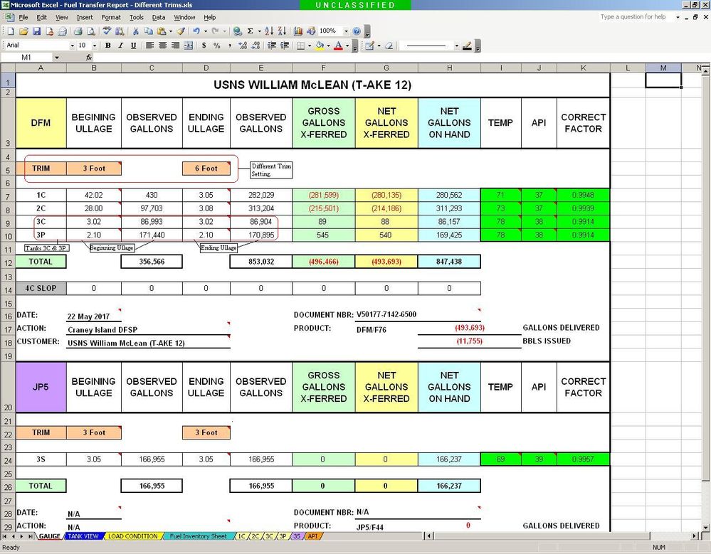
After getting everything setup I noticed a small glitch in the formulas for Trim.  I've attached the updated workbook and when you look at the Gauge tab you'll see two different Trim settings.  The problem is there are two tanks (3C & 3P) which have the same beginning and ending ullage because no fuel was transferred but due to the different Trims, the Observed Gallons are different.  This is normal and to be expected when the beginning and ending ullages are different but creates a false inventory when no fuel was actually transferred from those tanks.

If you could help me with the formula for those tanks (1C, 2C, 3C, and 3P) to default the Trim to "3 Foot" if the beginning and ending ullages are the same it would be greatly appreciated.

I'm sorry to keep asking you for help and this will be the last time because everything else works flawlessly with this workbook thanks to you and I didn't notice this error until late yesterday when getting everything in place and trying the different scenarios did it become apparent.

Again, thank you for everything!!!

[#11]

I'm sorry. I don't understand.

[#12]

Sorry for the confusion, I'll try again.  I've updated the previous request with cell references.

After getting everything setup and working the different Trim scenarios I noticed a small glitch in the formulas for Trim in the following cells (C7,C8,C9,C10,E7,E8,E9,E10).  I've attached the updated workbook and when you look at the Gauge tab you'll see two different Trim settings (B5 & D5).  The problem is there are two tanks (3C "A9" & 3P "A10") which have the same beginning ullage (B9 & B10) and ending ullage (D9 & D10) because no fuel was transferred but due to the different Trims, the Beginning Observed Gallons (C9 & D10) and Ending Observed Gallons (E9 & E10) are different.  This is normal and to be expected when the beginning and ending ullages are different but creates a false inventory when no fuel was actually transferred from those tanks; the readings in Gross Gallons X-Ferred (F9 & F10) and Net Gallons X-Ferred (G9 & G10) should be zero.

If you could help me with the formula for the tanks on this particular workbook (3C and 3P) to default to the Trim "3 Foot" since the beginning and ending ullages are the same it would be greatly appreciated.  What I mean by this is that since no fuel was actually transferred from those tanks (the beginning ullages (B9 and B10) and ending ullages (D9 and D10) are the exact same), the default Beginning Trim (B5) and Ending Trim (D5) should be 3 Foot.

If you could do just any one tank, say, 1C, I can modify the formula for the others.

The bottom half of the spreadsheet dealing with JP5 jet fuel works flawlessly since there is only one tank to work with.

Again, sorry for the confusion and hopefully this isn't confusing but if it is, please don't hesitate to ask.

Thank you again for the time your taking with this, it's greatly appreciated.

Gauge Tab with notes.

[#13]

Hi Detlef,

I took a break from looking at this and came up with a much shorter and hopefully less confusing version of this request.

If the Trim settings in cells B5 and D5 are different and the Beginning Ullage in cell B9 equals the Ending Ullage in cell D9, then I need the formula in cells C9 and E9 to default to "3 Foot" in cells B5 and D5 so I will get a zero in cells F9 and G9.

I've added your original formulas to the referenced cells below.

Cell C9 Formula
=INDEX('3C'!A:D,LOOKUP(B9,'3C'!A2:A342,ROW('3C'!C2:C342)),MATCH(B5,'3C'!1:1,0))

Cell E9 Formula
=INDEX('3C'!A:D,LOOKUP(D9,'3C'!A2:A342,ROW('3C'!C2:C342)),MATCH(D5,'3C'!1:1,0))

Again, thank you for your help with this.

[#14]

Wouldn't it be enough to change D5 from "6 Foot" to "3 Foot"?

[#15]

---

@Detlef Lewin wrote:

Wouldn't it be enough to change D5 from "6 Foot" to "3 Foot"?

---

Yes but only when B9 and D9 are equal to each other and B5 is already 3 Foot. The reason I'm asking for B5 also is because it could be 6 Foot or Even sometimes also.

I do apologize for the information overload so the following sentence is what I need your original formula modified to include, it's as concise as I can get it.

If B5 and D5 are not equal to each other and B9 and D9 are equal to each other then make B5 and D5 equal 3 Foot.  (This is so F9 and G9 will equal zero because no fuel was transferred from Tank 3C due to B9 and D9 are equal to each other.)

I've added your original formulas to the referenced cells below.  They work perfect as asked for when B9 and D9 are not equal to each other.

Cell C9 Formula
=INDEX('3C'!A:D,LOOKUP(B9,'3C'!A2:A342,ROW('3C'!C2:C342)),MATCH(B5,'3C'!1:1,0))

Cell E9 Formula
=INDEX('3C'!A:D,LOOKUP(D9,'3C'!A2:A342,ROW('3C'!C2:C342)),MATCH(D5,'3C'!1:1,0))

The following is a description of Trim for this class ship to help give you a picture of what's physically happening onboard that this spreadsheet represents.

"This class ship has three Trim conditions: Even, 3 Foot, and 6 Foot.  Normally we're at 3 Foot Trim most of the time which means the bow is three feet higher in the water than Even Trim or six feet higher in the water at 6 Foot.  When we issue a lot of fuel we can start out at 3 Foot Trim and end at 6 Foot trim because the fuel tanks are in the forward part of the ship and are now empty and the ballast tanks can't compensate enough to bring us back down to 3 Foot Trim.  For Even Trim (same as before we may start out at 3 Foot or 6 Foot, depending on how full the tanks are) we have loaded a lot of fuel that has caused the Trim to fall below the 3 Foot or 6 Foot Trim because the ballast tanks can't compensate enough to bring us up to 3 Foot Trim."

I hope I have cleared up the confusion and do apologize again for the earlier information overload.  I just wish I knew how to write the formula additions I have in bold to the formulas you've already provided; I've tried my best to simplify it to it's basic elements to what I need and added clarification for these unique scenarios.

I hope I haven't frustrated you with this, if so, then I do apologize, it wasn't my intent, only my lack of conveying my request to you in a clear and concise manner.

Please let me know if you need any further information, it's not a problem.

I do appreciate everything you've done for me,

[#16]

My idea is not the change a formula but use a new formula in F5.

=IF(AND(OR(B9=D9,B10=D10),B5<>D5),"Change D5 to '3 Foot'!","")

So the user in front of the sheet gets the instruction to change the value in D5.

And everything is balanced.

[#17]

---

@Detlef Lewin wrote:

My idea is not the change a formula but use a new formula in F5.

=IF(AND(OR(B9=D9,B10=D10),B5<>D5),"Change D5 to '3 Foot'!","")

So the user in front of the sheet gets the instruction to change the value in D5.

And everything is balanced.

---

Unfortunately this wouldn't work because it would change the values in the other tanks as well, but we're getting there.

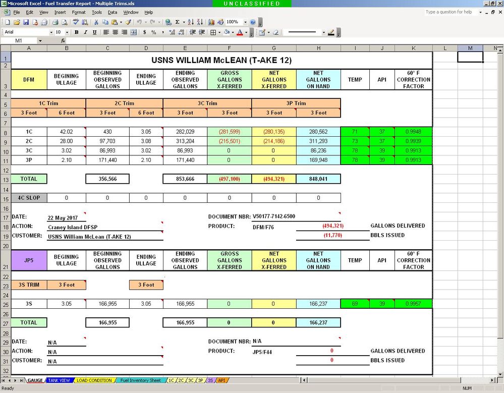
Instead of using your formula, I decided to add three more Trim Groups which accomplishes exactly what I needed.  I would've preferred to use just the two Trim cells but it looks like it's beyond Excel's design parameters.

I appreciate everything you've done for me, your help has been extremely invaluable, and the last formula you gave me provided the insight I needed to do to get this to work.  If in the future you find what I'm looking for, please let me know, it would be greatly appreciated.

As before, I still think your employer doesn't pay you enough because what you've done for me, you're worth you weight in gold a thousand-fold and then some.  If there was a way I could rate your help here, I would give you 10 out of 5 stars because you've gone well far and beyond what I could have ever expected with this ordeal.

Take care my friend,

John

Revised Gauge Tab

[#18]

In regards to your inquiry about creating a drop down selection list in excel.
Type the words Even, 3 Foot and 6 Foot (in three separate cells) on another area of your spreadsheet, then - once you're in the cell where you want the list - go to Data Tab>Data Validation dropdown>Data Validation>Allow dropdown>List>Data dropdown> Choose the list you typed earlier. Hit OK.

[#19]

Hello Detlef,

I'm in need of your help again. This time I only have one problem and not the entire workbook. Attached are the updated workbooks you helped me with last May. The one named 8039 Feet & Inches is the one I need updating and the other one is for comparison.

I need help with the following formula:

=INDEX('1C'!A:D,LOOKUP(E7,'1C'!A2:A509,ROW('1C'!C2:C509)),MATCH(B7,'1C'!1:1,0))

I need to be able to enter numbers in D7 and E7 and it will go to tab 1C and come up with the correct answer to put in F7 (based off the trim the MATCH portion of this formula provides. In this case the correct answer for 41 feet (in D7) and 2 inches (in E7) is 5,053 gallons in F7 and 3 Feet Beginning & Ending Trim.

If you can solve this one problem, I can edit the rest of the spreadsheet for the other tanks.

Thank you very much for your time with this.

Best Regards,

John

[#20]

Hello Detlef,

I’m in need of your help again; I’m pretty sure this is a much easier problem to fix since it’s only one problem and not the entire workbook.

I need help with the following formula:

=INDEX('1C'!A:D,LOOKUP(D7,'1C'!A2:A509,ROW('1C'!C2:C509)),MATCH(B7,'1C'!1:1,0))

I modified the spreadsheet recently and now I need the LOOKUP portion of this formula to include D7 and E7.  Originally D7 was feet and inches in a 2-decimal format but now feet and inches are in separate cells (D7 – feet and E7 – inches) in a regular number 0-decimal format.

This formula is used 20 times in this spreadsheet but if you can fix it for the one cell then I can edit the others myself.

I’m attaching both the current in-use workbook (8039 Decimal Format - Current) and the new in-progress workbook (8039 Feet & Inches - In Progress) for you to easily reference.

In the current in-use workbook all formulas and tabs are working as designed and you may notice a few changes in appearance since you last helped me last May.

In the new in-progress workbook all the cells and tabs have been updated to accommodate the new formula and is currently showing #REF! error codes due to on tab 1C, 2C, 3C, 3P, and 3S I changed the replaced the Ullage column with Ullage Ft and Ullage In columns.

If you have any questions, please don’t hesitate to ask.

Best Regards,

John