Excel formula assistance needed!

[thesspie_ann]

Hi all, 

I'm a bit of a novice when it comes to excel formulas, so any assistance I can get on the below would be amazing!

I need a formula that does the following: 

• On 1 sheet I have a table of numbers
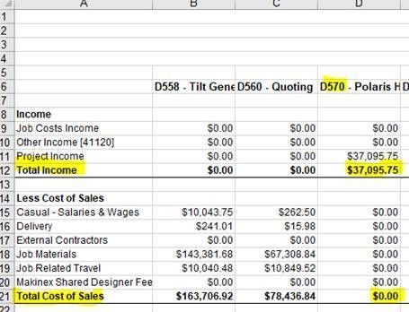
• The column headings contain a 3-digit job number (eg. D558 - General Tasks)
• Underneath each column heading there are rows titled ‘Total income’ and ‘Total cost of sales’
• On sheet 2 there is:
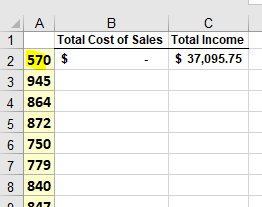
• A column with all the 3-digit job numbers from Sheet 1
• A column with the heading ‘Total income’
• A column with the heading ‘Total cost of sales’

I need formulas that fill the ‘total income’ and ‘total cost of sales’ columns in Sheet 2,

With the information in these corresponding cells in Sheet 1.

EG.

Sheet 1:

Sheet 1

Sheet 2:

Sheet 2

Let me know if any more info is required. 

Thank you!

[#2]

I am not good at Excel.  For this question, I can think of array formula solution only.

For Total Cost of Sales

=INDEX('Sheet1'!$B$6:$D$21, 2116, MATCH(TEXT('Sheet2'!$A2,"000"), MID('Sheet1'!$B$6:$D$6, 2, 3), 0))

where $D should be changed to the last column in your sheet1.

After typing the above formula, keep in the editing cell mode, press CTRL + SHIFT + ENTER to make it as a array formula. Then it will look like

{=INDEX('Sheet1'!$B$6:$D$21, 2116, MATCH(TEXT('Sheet2'!$A2,"000"), MID('Sheet1'!$B$6:$D$6, 2, 3), 0))}

For Total income

=INDEX('Sheet1'!$B$6:$D$21, 127, MATCH(TEXT('Sheet2'!$A2,"000"), MID('Sheet1'!$B$6:$D$6, 2, 3), 0))

remember to turn it to array formula.

Array formula has low performance issue.  If you data set is large, it performs slowly.

edition: correction is made in orange colour.

[#3]

Hi Willy, thanks so much for the reply!

I tried putting the formulas into the spreadsheet, but it comes up with #REF! when I click control + shift + enter. 

For total cost of sales, I edited the titles used so it looks like; 

=INDEX(ProfitLoss!$B$6:$FE$21, 21, MATCH(TEXT(Sheet1!$A2,"000"), MID(ProfitLoss!$B$6:$FE$6, 2, 3), 0))

The name of sheet 1 is actually 'ProfitLoss' and sheet 2 'Sheet1'. 

The last column is the spreadsheet is FE. 

I wasn't sure whether to change where it has '000' to the digits of the job number (eg. '570'), 

But when I did this it didn't give me the right number either. 

Any suggestions to where I've gone wrong?

Thanks!

[#4]

the 2nd parameter for index formula should be

7 for total income
16 for total cost of sales

I made mistakes before, sorry.

[#5]

Great, thanks WIlly!