Conditional formatting using different colours

[Russell pope]

I have a spreadsheet for work where there are dates (all different). I need to create a rule/s in conditional formatting so it highlights red when its due. Some are due every 2, 3 or four years.

I have the rule for yearly which is =NOW() 

But i don`t know how to flag it when its every 2, 3 or four years. 

05/10/2017

02/08/2014

26/05/2018

21/02/2017

[#2]

Can you describe more how you would like to highlight for yearly, every 2, 3 or 4 years?

Do you want this?
=YEAR(NOW())-YEAR(<theDateCell>)+1

[#3]

I would like it to highlight the cell red.

Example...if the date in the cell was 01/02/2014 and it was expired date say 3 years it would highlight red.

if that makes sense

[#4]

You may try this

=AND(DATEDIF($A1,NOW(),"y"),NOW())>=1,DATEDIF($A1,NOW(),"y"),NOW())<=4)

DATEDIF function can be found:

https://support.office.com/en-us/article/DATEDIF-function-25dba1a4-2812-480b-84dd-8b32a451b35c?ui=en...

[#5]

HI thanks for all your help. Unfortunately its still not working.

I can get it to highlight when it has expired after a year using =NOW() 

But i cannot get it to do the same for 2 years, 3 and four 

[#6]

The rule Willy gave returns TRUE if from now to start date is more than one year and less than four, and FALSE for any other dates.

If different rules (for 1,2,3 and 4 years accordingly) or number of years is set as a value (<n>) when it could be

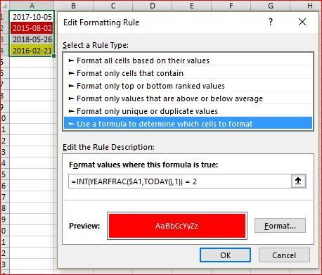
=INT(YEARFRAC(A1,TODAY(),1)) = <n>

[#7]

Thank you how would i input this, i`ve tried conditional formatting -- New rule -- Use a formula to determine which cells to format.

or is there another way?

I would like to say thank you for everyone's help 

[#8]

Hi Russell,

Yes, new rule->use a formula, the only point is to use correctly absolute and relative references in formula. If you apply the rule to the column use like $A1, if to the row like A$1, etc. 

[#9]

Thank you so how would I wright the formula if the cell was say E24.

Sorry if this is taken to much time

[#10]

Russel,

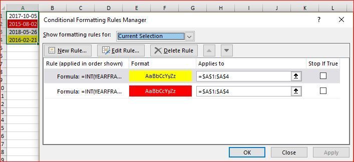
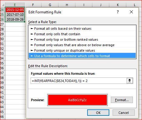
Not sure what is E24, let say your dates are in column A and you apply the rule (red) for due date over 2 years

and the same for 1 year (=1) in yellow, applying to your range

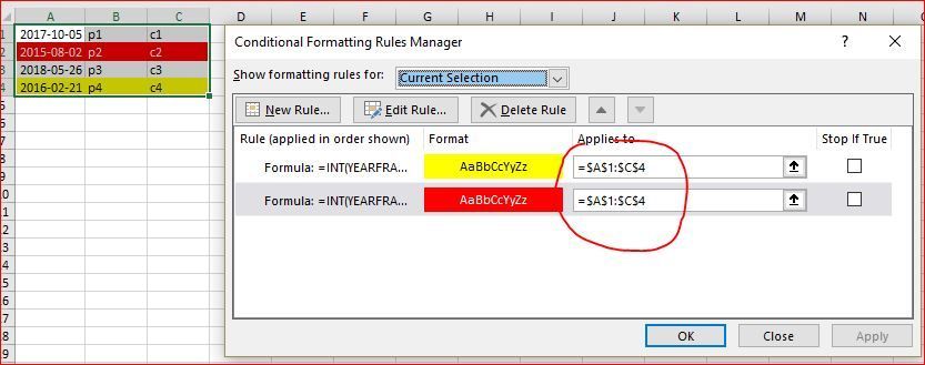
Using $A1 in the rule means you compare each cell in column A applying it to you range.

If you expand your range and apply it to expanded range still compare $A1 rules highlight entire row in the range

[#11]

Sorry what I meant was say cell E24 had the date 12/05/2015, cell E25 has 07/10/17, cell E26 26/09/18 and each cell will highlight red when it has expired 2 years

So for 07/10/17 it will highlight red on 07/10/19

So how would the formula be written?

[#12]

Russel, formula is the same if i understood you correctly

for today only first date is highlighted since it's 2 years over.

[#13]

Thank you.

How would i wright it for individual boxes and just compare it to today's date?