- Home
- Microsoft 365
- Excel
- Conditional Formatting based on Separate Column
Conditional Formatting based on Separate Column
- Subscribe to RSS Feed
- Mark Discussion as New
- Mark Discussion as Read
- Pin this Discussion for Current User
- Bookmark
- Subscribe
- Printer Friendly Page
- Mark as New
- Bookmark
- Subscribe
- Mute
- Subscribe to RSS Feed
- Permalink
- Report Inappropriate Content
Feb 07 2018 10:53 AM - last edited on Nov 09 2023 11:10 AM by
HI, I'm new to excel formulas and conditional formatting! I'm using a spreadsheet to track new hires, and I'm trying to figure out how I can use "less footsteps" and not have to apply conditional formatting to every.single.cell. in a column..... I'd like to be able to type in something into my "L" column, and have the "D, M, N & O" columns to change color based on what is typed. I know that I can go in and individually click on the cells and then conditionally format them, but I'm going to have well over 300 different entries that I'm going to be working with. I'd love to get that time back! I've tried searching on this forum but can't find what I'm looking for....Thanks for your help! I've attached a snip to show what I'm working with. :)
- Labels:
-
Formulas & Functions
-
Show and Tell
- Mark as New
- Bookmark
- Subscribe
- Mute
- Subscribe to RSS Feed
- Permalink
- Report Inappropriate Content
Feb 07 2018 05:21 PM - edited Feb 07 2018 05:30 PM
From your screenshot, I do not know when "New Hire" and those column should be highlighted.
I think, if you are new to excel, you may not have the ideas of "Relative Reference", "Absolute Reference" and "Mixed Reference".
Using Contional Formatting, in the rules, you can use the mixed reference address. For example, I guess you want to highlight Column M whenever Column L is "Transfer". Your conditional formatting rule in Column M can be do it in this way:
- Select M2 (The cell at row 2 in column M)
- Home > Styles > Conditional Formatting > Manage Rules
- New Rule
- "Use a formula to determine which cells to format" (you probably have done it)
- This step is one of the key that you need to know. You can type the following formula
=$L2="Transfer"
The above formula is using Mixed reference address.
- Apply the format you want
- Click ok button
- Now, you should be still in Conditional Formatting Rules Manager dialog. You can see "Applies to", you can select the cells that you want the rule applies to, i.e. $M$2:$M$100.
- click ok.
In the above steps, step 5 and 8 are related to each other. In step 5, the formula locks Column L, but not locks on rows. If that formula apply to another row, e.g. applying on M3, the formula will actually becomes
=$L3="Transfer"
and now, step 8 says that the rule (you may think of the formula) is going to apply on M2 to M100. The rule will have adjustment according to the rows. Hence, 1 conditional formatting rule can apply to 99 cells in column M from row 2 to row 100.
You try to update your rules to see if it is the "less footsteps" approach.
- Mark as New
- Bookmark
- Subscribe
- Mute
- Subscribe to RSS Feed
- Permalink
- Report Inappropriate Content
Sep 12 2023 02:04 PM
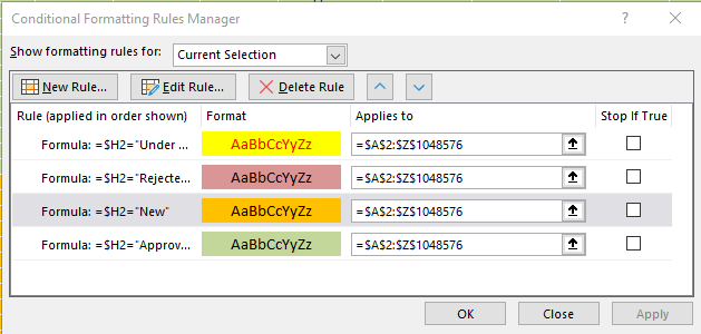
I think this is what you are looking for:
Based on a content of Column "H" the cells from "A2" to "Z1048676" filled with selected color.
If you want use only a single cell, just fix it: Instead of $H2 use $H$2 (replace with your specific cell)
- Mark as New
- Bookmark
- Subscribe
- Mute
- Subscribe to RSS Feed
- Permalink
- Report Inappropriate Content
Feb 06 2024 04:48 PM
