no subject

[jeremy_klip]

good day

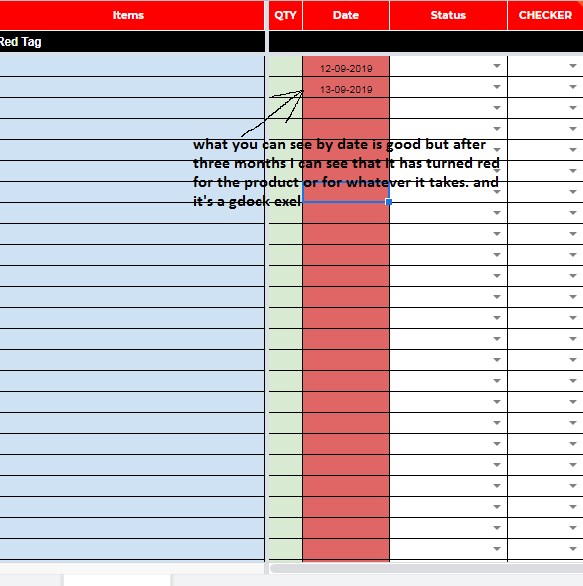
How can I look up a formula or get advice. When I enter a date in the sheet I want to see after three months that it has turned red. I work as a red tag and ensure that goods are sent back after three months.
Greetings Jeremy
j.klipje@outlook.com

[#2]

@jeremy_klip 

Apply a conditional format with the formula

=  EDATE(date,3)<TODAY()

where 'date' is a relative reference to the current cell.

[#3]

@Peter Bartholomew 

i think that i make worst bycause it dont work. maybe i make mistake whit the formule but if i put date 12-9-2019 en i hope about three monts its bycaumse red but nothing works 

[#4]

@jeremy_klip 

Please find the attached with a conditional formatting applied to the range A2:A100 with the formula...

=AND(ISNUMBER(A2),EDATE(A2,3)<TODAY())

As per the formula, if there is a date in column A and once today's date is greater than the date 3 months after the date entered in column A, the date in column A would turn red with white and bold/italic font. In other words, the date in column A would turn red after 3 months.

Please refer to the attached for more details.

[#5]

@Subodh_Tiwari_sktneer 

You cain see what i mean about 

[#6]

@jeremy_klip 

The suggested conditional formula will do the dame thing.'

e.g. if the date you entered is 12/09/2019 (dd/mm/yyyy), it will turn red after the date 12/12/2019. Isn't it what you are trying to achieve?

All you need is to apply the conditional formatting similar to one in the file I uploaded and you only need to change the formula used for conditional formatting as per your date column.

In the sample file, I assumed that the dates are in column A and start from Row#2 and applied the conditional formatting based on the formula =AND(ISNUMBER(A2),EDATE(A2,3)<TODAY()).

So if in your original workbook, the dates are in column D and they start from Row#3, all you need is to select the range starting from D3 and apply a new rule for conditional formatting using the formula given below and set the format as per your choice.

=AND(ISNUMBER(D3),EDATE(D3,3)<TODAY())

If you still have difficulty in implementing the conditional formatting, upload a sample workbook so that we can help you to do that.