help with IF statement...

[gms4b]

I have a laboratory instrument which spits out mostly numbers, but occasionally a phrase, such as "N/A" or "No Peak" or "<0". However, I needed a column in excel that only contained numbers...so I made this formula to convert any of these statement to "0" in the neighboring column:

=IF(INDIRECT(background!$B$3 & "2:"&background!$B$3 & "245")="No Peak",0,IF(INDIRECT(background!$B$3 & "2:" & background!$B$3 & "245")="N/A",0,IF(INDIRECT(background!$B$3 & "2:"&background!$B$3 & "245")="< 0",0,INDIRECT(background!$B$3 & "2:"&background!$B$3 & "245"))))

(the INDIRECT portion cobbles together a column letter and a number from a phrase it searches for on another tab. I don't think that's relevant here,...just the IF statement).

And it works fine, But, the instrument also spits out the phrase "#DIV/0!" and Excel doesn't know what to do with it....it just provides the phrase again in the formula column. Any ideas how I can get this phrase to convert to "0" properly?

[#2]

@gms4b , you may wrap your formula with IFERROR

=IFERROR(<formula>,0)

[#3]

@gms4b 

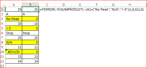
Perhaps entire formula

=IFERROR( IF(SUMPRODUCT(--(INDIRECT(background!$B$3 & "2:"&background!$B$3 & "245")={"No Peak","N/A","< 0"})),0,INDIRECT(background!$B$3 & "2:"&background!$B$3 & "245")),0)

[#4]

@Sergei Baklan 

AhHa! So I simply did this and it worked to take out the #DIV/0! statement and turn it to a 0. The remainder of the formula still converts the other statements to 0. 

I'm not sure what's going on with the other formula but its not really working right. I think it was giving 0's for everything...including normal numbers. 

Thanks for your help!!

Greg

[#5]

@gms4b 

Hi Greg,

Please check attached how it works in this sample

[#6]

@Sergei Baklan 

Thanks Sergei...I will keep playing with it. If I use your formula and put in the direct cell then things do work correctly. When I substitute in the INDIRECT portion instead of the direct cell name then it breaks and just gives me 0. 

I'll play with it again tomorrow....time to pick kids up from school.

Thanks,

Greg

[#7]

@gms4b 

Greg, I missed what INDIRECT() returns range, not the cell. If so simply wrap the formula by IFERROR like

=IFERROR(IF(A1:A12="No Peak",0,IF(A1:A12="N/A",0,IF(A1:A12="< 0",0,A1:A12))),0)

to optimize it it desirably to know more details of how your data is structured. It looks like you return the value from background sheet into the current row by row, from row 2 to row 3, from 3 to 3, etc and column by column. But I'm not sure.

[#8]

@Sergei Baklan 

Yeah, I think I'll just keep with wrapping my old formula in IFERROR like you suggested. That works well!

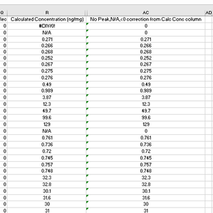
I think you're correct in your assessment. Column R in my spreadsheet contains all the data including several text terms......but I need the column to only contain numbers - and that is accomplished in column AC. The original formula converted most of the terms to 0 (like N/A) but not #DIV/0!. Wrapping the formula in IFERROR took care of that as you can see (for R2--->AC2). 

So, there's an INDEX function elsewhere that looks for a certain word ("calculated concentration (ng/mg)") from a column header and returns the column number that it is in and then converts it into the column letter (in the "background" sheet). That letter (in this case it's R) is then referenced in the formula's INDIRECT statement to point to a range of cells......so, R2:R245 for instance. 

Using the entire range in the formula still returns the result from the corresponding row when you cut/paste the formula from row 2 to 245 (i.e. the formula doesn't seem to need the exact cell number). But, maybe that's how its supposed to work. I'm not an Excel expert, in fact, I'm pretty sure that someone from this forum helped me with this formula!

I guess the problem is that I need to have the INDIRECT command in there because in my next data set the data could be in column S or U or somewhere else...it could change. 

Cheers,

Greg

[#9]

@gms4b 

Greg, it's not necessary to use INDIRECT, you already return needed column number, use it on INDEX for entire sheet like

=IFERROR(
    IF(
       SUMPRODUCT(--(INDEX(background!A:Z,ROW(),MATCH(Sheet1!B$1,background!$1:$1,0))={"No Peak","N/A","< 0"})),
       0,
       INDEX(background!A:Z,ROW(),MATCH(Sheet1!B$1,background!$1:$1,0))
    ),0)