Vlookup and return entire row from another sheet

[Maeby]

Is it possible to get VLOOKUP to return an entire row of data from a second sheet? I admit that I'm not the most skilled in Excel but I've been trying my best for hours now and would greatly appreciate some help.

In my case it looks like this:

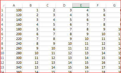
On my primary sheet, I want to be able to enter a profile number and then retrieve an entire row of cells with data related to it from another sheet, is this possible?

English isn't my first language so I'll post images for clarification.

In the images it would be entering the value 260 on my primary sheet and wanting all of row 25 (from B to AA) on the secondary sheet to be pasted next to it.

[#2 · Accepted solution]

@Maeby While this can be accomplished with VBA, if you're in the Insider program, you can use the FILTER() function.

If your data in Sheet2 is in rows A:BB, and there are 260 rows on that table, and you were trying to use a value in B3 to perform the lookup, the formula would be:

=FILTER(Sheet2!$A$2:$BB$260,Sheet2!$A$2:$A$260=B3,0)

This formula says to return all rows (from the table in Sheet2) where the values in column A equal the value in B3. 

Unfortunately, this feature is only currently available with the insider program in O365, but this is the way that the formula would work!

[#3]

I noticed that, in your image for Sheet1, you entered 260 under Type rather than under Profile. I shall assume you intended to enter 260 under Profile, such that this formula in B3 returns the data (starting with Type) corresponding to Profile 260:
=VLOOKUP($A3,
Sheet2!$A3:$AA100,
COLUMN(),0)
Note that the foregoing formula assumes both Sheets to have the same structure; otherwise, modify COLUMN() to this:
MATCH(B$2,Sheet2!$A$2:$AA$2,0)

[#4]

@Maeby 

One more variant - for data like this in Sheet2

in C3 of Sheet1

is

=IFERROR(INDEX(INDEX(Sheet2!$A$1:$AA$100,MATCH($B$3,Sheet2!$A$1:$A$100,0),0),1,COLUMN()-COLUMN($B$3)+1),"")

and drag it to the right.

[#5]

@Maeby 

Again Office 365 insider ...

XLOOKUP will return an entire row as a reference

= XLOOKUP( required, Type, profile, "" )

[like @Twifoo I am not sure whether one looks up a type to find a profile or the other way round]

Hopefully VLOOKUP will soon be consigned to the trash can of history where it belongs but, to be fair to it, it will return an array of values if given an array of column offsets

= VLOOKUP( required, Table, SEQUENCE(1,26, 2), 0 )

I have chosen to use a dynamic array function but hard-wired indices will do the job just as well.

[#6]

The workbook is for steel beams so the profile in that example was HEA, there are multiple profile sheets, I just didn't enter anything there since it wasn't really relevant. The main sheet is calculations based on the data from the others. thanks for the response tho

[#7]

Still working on learning VBA but in the meantime, this was a great answer that will save me loads of time, thank you! I'll re-sign (odd word in this context) to the insider program and give it a shot!  @macrordinary