Using Data in one field to fill check boxes or add yes or no into other fields.

[Frazz4real]

I am adding new users from a web page, the information populates to a spreadsheet. That works just fine. One of the fields that populates is the position field. There are a number of possible options here as youd imagine. Each position is assigned certain things, emails, cell phones, laptops. So what I would like to have happen is have excel read the contents of the position cell and populate other columns with yes or no. 

so if the position is Executive Director G2 would read ED. then H2 will be email, Ix will be cellphone, and so on. I am trying to set up a long function  that says if G2 = ED then H2, yes, I2, yes, etc. 

The difficulty is there are 12 possible positions each one needs to have different yes and no answers to the email, cellphone, laptop questions.

Anyone have a solution to this? I am not coming up with one. 

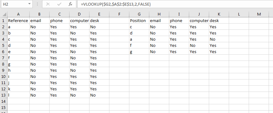
[#2 · Accepted solution]

If you have a reference table (i.e. a table with the 12 positions along the first column and the Yes/No responses in each of the following columns) you can use the vloolup function to do this. I have made a sample sheet that you can use as a reference. 

[#3]

could these be put on separate sheets? the reference and the actual data about the employee. 

The goal is to have the Manager at a location in our enterprise go to a web site enter the name, number, location, and position of the new employee and then use the position abbreviation as the reference value. For us in IT we would want to see all that information, plus what hardware they need and what applications they need to be setup in. So what if sheet 2 had the references and sheet 1 called them?

what would that look like with Vlookup?

[#4]

Hi @Frazz4real,

This can be handled using a MATCH & VLOOKUP function. This looks a bit insane, but it's not as complicated as it seems, so please bear with me. I included my file so you can see exactly what I did.

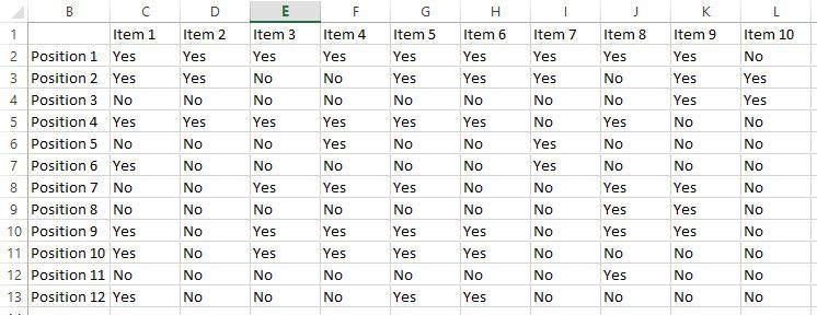
On one sheet, I created a matrix with the positions listed down the left, the items across the top and a yes or no for each position/item combo. (I started on B in this example):

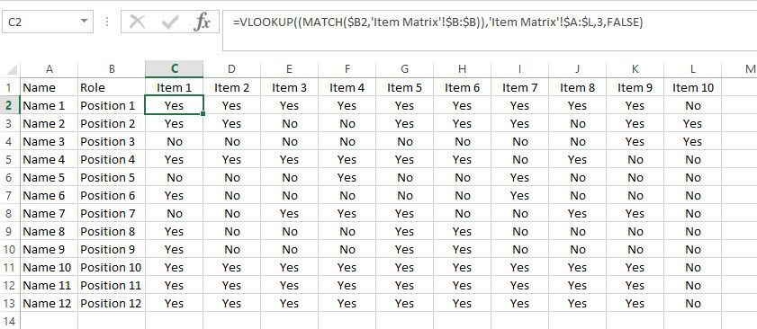
On another sheet, I have a column that shows the employee name in column A and their position in column B. I copied the item row and pasted it across the top. What I want to do is create a formula for each item that's going to look at the role and the item, then search the matrix to see if that role gets that item. This is where I used the MATCH & VLOOKUP functions. It's a bit of a hassle for one row, but then you can copy the formula to all of the cells and it'll calculate correctly.

Starting with the first item for the first person, I used formula: =VLOOKUP((MATCH($B2,'Item Matrix'!$B:$B)),'Item Matrix'!$A:$L,3,FALSE)

I started with MATCH simply to determine which row the position was on:

• Lookup value: click in the cell of the first position and add a $ before the column to lock the match to that column since we're going to be pasting this formula across - that way it will always look in the position row. I entered $B2 since I want to lock the column, but not the row.
• Lookup array: select the row on your matrix where the positions are listed. Again, place a $ before the columns to lock the lookup to just that column. I entered $B:$B to only look in column B

Next, I created my VLOOKUP formula. You're going to do this once, then paste it to each column updating just 1 value, so it should be decently easy to do:

• Lookup value: my MATCH formula in parentheses - this tells VLOOKUP which row to search
• Table array: I selected all the columns that contained my matrix info. You can select just the matrix, but if you end up adding more positions, this will make it so you don't have to update your formulas, just the matrix. Add the $ to lock the lookup to those columns. I entered Sheet6!$A:$L to search columns A-L.
• Col Index #: This is the column that corresponds to the item you're looking up. Since I'm starting with item 1 which is in column 3, I enter 3. This is the value you will need to change for each column you paste this formula into; everything else will remain the same.

Once you've entered this formula for the first person/first item, ensure the answer is correct. Then, copy and paste the formula across the first row for the first person. Now you'll need to update the Col Index No for each column. Mine started with a col index value of 3 in column C, so in column D, I'll need to update that to 4. In column E, I'll change it to 5, in F I'll change it to 6 and so on until I've reached the end.

Now, I can just copy that first row of formulas and paste them down the columns for each person and the formulas will auto-update showing the correct info for the correct person and position.

I hope this helped you accomplish what you want to do!

[#5]

Thank you, This is exactly what I need.