Taking values from certain rows based on data input

[Drakerla]

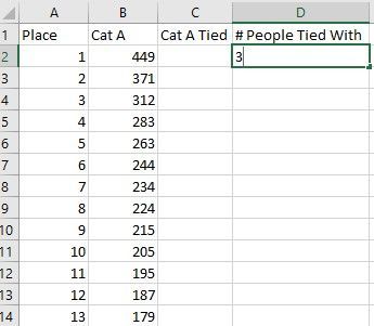
So I'm trying to get a value into the column "Cat A Tied" (C column). This value depends on the number in the "# People Tied With" column (D Column). In this case, cell D2 has the number 3 in it. I want the sum of the first three rows of the B column (not including column headers) and then divide that by 3. However, I want the cell to be dynamic so if I change the number to 5 it will then automatically take the sum of the first 5 rows and divide by 5. Additionally, if I put this value into D3, the second row of my table, I'd want the first number (3 or 5, or any number put in) of rows from that same row onwards instead of from the first row of the data set.

Any help would be greatly appreciated :)

[#2]

@Drakerla 

Please try this and let me know if this is what you are trying to achieve.

In C2

=IF(D2="","",SUM(OFFSET($B$1,ROW(D2)-1,,D2)))

and then copy it down.

[#3]

@Subodh_Tiwari_sktneerYes that's brilliant! Thanks so much!
Would you mind explaining how it works please, as I like to learn these things for future use?

[#4]

The only change needed is to divide that SUM value by the value in cell D2. But thank you so much for your help!

=IF(D2="","",SUM(OFFSET($B$1,ROW(D2)-1,,D2)))/D2

[#5]

@Drakerla 

It seems I missed the division part but that was easy to fix and glad you did it right.

The range passed to the SUM function is derived with the help of OFFSET function in which the anchor cell is $B$1 (which is absolute reference and will always be the same when you copy the formula down) and the row is offset by ROW(D2)-1 which returns the first cell in the sum range i.e. if the formula is placed in the second row, ROW(D2)-1 will return 1 and hence the first cell in the sum range would be one row offset from the anchor cell B1 which would be cell C1 (if you wish you may remove the D2 from ROW(D2) and make it just ROW() and it will work in the same way) and then the height is determined by the number in the D2, If you evaluate the formula in D2, it would be easy for you to know how this formula works.

If that takes care of your original question, please accept the post with the proposed solution as a Best Answer/Response to mark your question as Solved.

[#6]

@Drakerla 

Another variant

=IFERROR(SUM(INDEX(B:B,ROW()):INDEX(B:B,ROW()+$D2-1))/$D2,"")