- Home
- Microsoft 365
- Excel
- Limit chart data displayed in excel
Limit chart data displayed in excel
- Subscribe to RSS Feed
- Mark Discussion as New
- Mark Discussion as Read
- Pin this Discussion for Current User
- Bookmark
- Subscribe
- Printer Friendly Page
- Mark as New
- Bookmark
- Subscribe
- Mute
- Subscribe to RSS Feed
- Permalink
- Report Inappropriate Content
Jun 25 2019 12:06 PM
I have a chart with 2 data series: YTD Budget and YTD Received. Both the YTD Budget and YTD Received data are in running total columns. I manually enter the weekly amount Received.
The current week number is in Cell M1. The Week Beginning Date is displayed by the following formula: =VLOOKUP($M$1,$M$5:$W$57,2,FALSE)
Row 5 is Week 1, and Row 56 is the last week for 2019.
All the YTD Budget data points should be displayed, but I only want the non-zero YTD Received data points displayed.
The Series Values for Received is: =Sheet1!$U$5:$U$56
"$U$56" displays ALL 52 weeks of YTD Received amounts, but I want to end the series at the last week that has data in the Received column.
Can I use current week number is in Cell M1 to limit the Series Values?
Thank you for your help.
- Labels:
-
Excel
- Mark as New
- Bookmark
- Subscribe
- Mute
- Subscribe to RSS Feed
- Permalink
- Report Inappropriate Content
Jun 25 2019 12:50 PM - edited Jun 25 2019 12:51 PM
Solution
hi,
In cell M1 I generated the week number by using the formula
=Weeknum(Today())
For the line Chart to reflect the values only until this week (say week 26) you need to define 2 names:
I called them Received & Budget
You do that by hitting CTRL + SHIFT + F3
Name: Received
Refers To: =OFFSET(Sheet1!$U$5,0,0,Sheet1!$M$1,1)
Name: Budget
Refers To: =OFFSET(Sheet1!$W$5,0,0,Sheet1!$M$1,1)
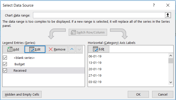
Now we need to modify the data used for the Line Chart >> Select it >> Design Tab >> Select Data
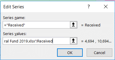
Select the series "Received" >> Edit >> Replace the range reference by the Defined Name "Received" without deleting the sheet name or the exclamation mark
Repeat for the Budget Series
Now after hitting OK twice the Line Chart will only reflect the valid period
If you want to deal with Zero values then in the select Data Source box >> Click in the lower Left corner >>Hidden and Empty Cells >> select one of the options
I am attaching the file for your reference
Hope that helps
Nabil Mourad
- Mark as New
- Bookmark
- Subscribe
- Mute
- Subscribe to RSS Feed
- Permalink
- Report Inappropriate Content
Jun 27 2019 10:31 AM
Accepted Solutions
- Mark as New
- Bookmark
- Subscribe
- Mute
- Subscribe to RSS Feed
- Permalink
- Report Inappropriate Content
Jun 25 2019 12:50 PM - edited Jun 25 2019 12:51 PM
Solution
hi,
In cell M1 I generated the week number by using the formula
=Weeknum(Today())
For the line Chart to reflect the values only until this week (say week 26) you need to define 2 names:
I called them Received & Budget
You do that by hitting CTRL + SHIFT + F3
Name: Received
Refers To: =OFFSET(Sheet1!$U$5,0,0,Sheet1!$M$1,1)
Name: Budget
Refers To: =OFFSET(Sheet1!$W$5,0,0,Sheet1!$M$1,1)
Now we need to modify the data used for the Line Chart >> Select it >> Design Tab >> Select Data
Select the series "Received" >> Edit >> Replace the range reference by the Defined Name "Received" without deleting the sheet name or the exclamation mark
Repeat for the Budget Series
Now after hitting OK twice the Line Chart will only reflect the valid period
If you want to deal with Zero values then in the select Data Source box >> Click in the lower Left corner >>Hidden and Empty Cells >> select one of the options
I am attaching the file for your reference
Hope that helps
Nabil Mourad

